Working Paper No. 421
A Simplified Stock-Flow Consistent
Post-Keynesian Growth Model
by
Claudio H. Dos Santos* and
Gennaro Zezza**
*The Levy Economics Institute
**The Levy Economics Institute and University of Cassino, Italy
April 2005
We would like to thank Duncan Foley, Wynne Godley, Marc Lavoie, Anwar Shaikh, Peter Skott, and Lance Taylor for commenting on previous versions of this paper. The remaining errors in the text are all ours, of course
The Levy Economics Institute Working Paper Collection presents research in progress by Levy Institute scholars and conference participants. The purpose of the series is to
disseminate ideas to and elicit comments from academics and professionals.
The Levy Economics Institute of Bard College, founded in 1986, is a nonprofit, nonpartisan, independently funded research organization devoted to public service. Through scholarship and economic research it generates viable, effective public policy responses to important economic problems that profoundly affect the quality of life in the United States and abroad.
The Levy Economics Institute P.O. Box 5000
Annandale-on-Hudson, NY 12504-5000 http://www.levy.org
In a series of papers (e.g. Zezza and Dos Santos, 2004; Dos Santos, 2004a, 2004b) we
have argued that the so-called “stock-flow consistent approach” (SFCA) to
macroeconomic modeling not only provides a rigorous foundation for post-Keynesian
macroeconomics but is also a relatively unexplored frontier of (various schools of)
Keynesian macroeconomics1.
We have noted also that the increase in analytical rigor allowed by the SFCA does
not come without a price. More often than not, SFC models are too big to be analytically
treatable and can only be analyzed with the help of computer simulations. Since the
“reality” post-Keynesian SFC models try to approximate is complex, this is hardly
surprising2. On the other hand, we do acknowledge that an analytically treatable version of our models would help the presentation of our ideas considerably. This paper aims
precisely to present one such version.
In fact, we believe that the model presented here—which builds on previous
efforts by Godley and Cripps (1983), Godley (e.g. 1996, 1999), Lavoie and Godley
(2001-2002), Taylor (1991), and Tobin (e.g. 1980, 1982), among others—is intuitive and
general enough to be considered a “baseline” (didactic) SFC post-Keynesian model3. As we hope to make clear to the reader, it sheds light on a wealth of classic post-Keynesian
macroeconomic issues, and (just like the old IS/LM model) can easily be modified to
address several other ones (or the previous ones from different theoretical perspectives).
What follows is divided in four parts. First we present the “structural” hypotheses
of the model and the logical (accounting) constraints imposed by them. Second, we
“close” the accounting constraints with a specific set of post-Keynesian behavioral
hypotheses4. Third, we discuss the “short period” and “long period” properties of our specific “closure.” We finish with a brief discussion of possible extensions and
simplifications of the model.
1
Essentially the same points were noted well before us—with different terminologies—by Tobin (1980, 1982), Godley and Cripps (1983), and Lavoie and Godley (2001-2002), among others.
2
The adjective post-Keynesian is used here in the sense of Palley (1996) and Lavoie (1992).
3
Conceived as a simplified version of Zezza and Dos Santos (2004), the model presented here ended up being very close in spirit to “the” “heterodox model” by Foley and Taylor (2004).
4
1. THE STRUCTURE OF OUR ARTIFICIAL ECONOMY
The economy assumed here has households, firms (which produce a single good, with
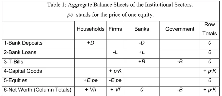
price p), banks and a government sector5. The aggregated assets and liabilities of these institutional sectors are presented in table 1 below.
Table 1 summarizes several theoretical assumptions. First and foremost, the
economy assumed here is a “pure credit” one, i.e. all transactions are paid with bank
checks6. Moreover, the banking sector is supposed to remunerate deposits at the T-bill rate (making profits only through their loans to firms), so households do not care to buy
T-bills themselves, keeping their wealth only in the form of bank deposits and equities7. The banking sector is also assumed to: (i) accept government debt as means of payment
for government deficits8; (ii) not pay taxes; and (iii) to distribute all its profits (so its net worth is equal to zero)9. Finally, firms are assumed to finance their investment using loans, equity emission and retained profits. The Modigliani-Miller (1958) theorem does
not hold in this economy, so the specific way firms choose (or find) to finance themselves
matters and their net worth is not necessarily zero (i.e. Tobin’s q is not necessarily 1)10.
5
Dos Santos (2004b) argues that these are quintessential features of the economies studied by “Financial Keynesian” authors (such as Davidson, 1972; Godley, 1999; Minsky, 1986; and Tobin, 1980). Similar economies have been studied in a long series of papers by Reiner Franke, Willi Semmler, and associates, at least since Franke and Semmler (1989).
6
A similar simplifying hypothesis is adopted in Godley and Cripps (1983, chapter 5). Section 4 discusses the implications of relaxing it.
7
According to Stiglitz and Greenwald (2003, p.43), a banking sector with these characteristics “is not too different from what may emerge in the fairly near future in the USA.” In any case, this hypothesis allows us to simplify the portfolio choice of households considerably. More detailed treatments (such as the ones in Tobin, 1980; or Lavoie and Godley, 2001-2002) can easily be introduced, though only at the cost of making the algebra considerably heavier (see section 4 for a discussion).
8
Here we will work with the conventional case in which B>0, noting that not too long ago (in the Clinton years, to be precise) many analysts were discussing the consequences of the U.S government paying all its debt. A negative B (i.e. a positive government net worth) would be interpreted in this model as “net central bank advances” to the banking sector as a whole.
9
We are also simplifying away banks’ (and government’s) investment in fixed capital, as well as their intermediary consumption (wages, etc). These assumptions are made only to allow for simpler mathematical expressions for household income and aggregate investment.
10
Table 1: Aggregate Balance Sheets of the Institutional Sectors.
pe stands for the price of one equity.
Households Firms Banks Government Row
Totals
1-Bank Deposits +D -D 0
2-Bank Loans -L +L 0
3-T-Bills +B -B 0
4-Capital Goods +p·K +p·K
5-Equities +E·pe -E·pe 0
6-Net Worth (Column Totals) + Vh + Vf 0 -B + p·K
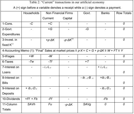
Table 2 below shows the “current flows” associated with the stocks above. As such, it
(rigorously) represents very intuitive phenomena11. Households in virtually all capitalist economies receive income in the form of wages, interest on deposits, and distributed profits (of
banks and firms) and use it to buy consumption goods, pay taxes and save (as depicted in the
households’ column of table 2)12. The government, in turn, receives money from taxes and uses it to buy goods from firms and pay interest on its (lagged stock of) debt, while firms use sales
receipts to pay wages, taxes, interest on their (lagged stock of) loans, and dividends, retaining the
rest to help finance investment. Finally, banks receive money from their loans to firms and
holdings of Treasury bills and use it to pay interest on households’ deposits and dividends. In a
“closed system” like ours every money flow has to “come from somewhere and go somewhere”
(Godley, 1999, p.394), and this shows up in the fact that all row totals of table 2 are zero.
11
A numerical example in section 3 aims to provide further assistance to the reader in understanding exactly how the artificial economy presented here operates.
12
Table 2: “Current” transactions in our artificial economy
A (+) sign before a variable denotes a receipt while a (-) sign denotes a payment.
Households Non Financial Firms
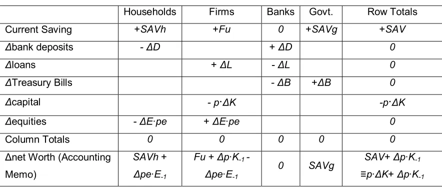
If it is true that beginning of period stocks necessarily affect income flows (and,
as we shall see, asset prices), it is also true that saving flows and capital gains necessarily
affect end of period stocks15. This is shown in table 3. Given the hypotheses above, households’ saving necessarily implies changes in their holdings of bank deposits and/or
stocks, while government deficits are necessarily financed with the emission of T-bills,
13
We follow here the broad Keynesian literature in simplifying away investment in inventories (which plays a crucial role in Godley and Cripps, 1983 and Shaikh, 1989). These can be easily introduced (say, along the lines of Godley, 1999), though only at the cost of increasing the complexity of the model.
14
Firms’ investment expenditures in physical capital imply a change in their financial or capital assets and, therefore, is a “capital” transaction. As such it (re)appears in table 3 below. The reason it is included in table 2 is to stress the idea that firms buy their capital goods from themselves, an obvious feature of the real world (though a slightly odd assumption in our “one good economy”) .
15
and investment is necessarily financed by a combination of retained earnings, equity
emissions and bank loans. As emphasized by Godley (1999), the banking sector plays a
crucial role in making sure these inter-related balance sheet changes are mutually
consistent16.
Table 3: Flows of Funds in our artificial economy
Positive figures denote sources of funds, while negative ones denote uses of funds.
Households Firms Banks Govt. Row Totals
Current Saving +SAVh +Fu 0 +SAVg +SAV
Before we continue, we must remind the reader that all accounts presented so far
were phrased in nominal terms. All stocks and flows in tables 1 and 2 above have
straightforward “real” counterparts given by their nominal value divided by p (the price
of the single good produced in the economy), while the “real” capital gains in equities are
given by:
∆pet·E-1/pt – ∆p·pe-1E-1/p-1·pt;
and the “real” capital gains in any other financial asset Z are given by:
- ∆p·Z-1/p-1·pt17.
16
As is well known, most macroeconomic models assume that some sort of Walrasian auctioneer takes care of financial intermediation. We believe this simplification is not faithful to the views of financially
sophisticated post-Keynesians (such as Davidson, 1972; Godley and Cripps, 1983; and Minsky, 1986), though.
17
2. A FIX-PRICE SIMPLIFIED POST-KEYNESIAN CLOSURE
We shall work here with a simplified “fix-price” version of the model, leaving the
discussion of extensions to part 4.
2.1Aggregate Supply
Following Taylor (1991, chapter 2), we assume that:
(E1) p = w·b·(1+τ);
where p =price level, w = money wage per unit of labor, b = labor-output ratio, and τ = mark up rate. From (1) it is easy to prove that the (gross, before tax) profit share on total
income (π) is given by:
(E2) π = [p·X - W]/p·X = τ/(1+τ);
so that the (before tax) wage share on total income is:
(E3) 1 - π =W/ p·X = 1/(1+τ);
and W = (1 – π)·p·X.
We assume here that the price level, the technology, and the income distribution of the
economy are exogenous, so all lower case variables above are constant (i.e. the aggregate
supply of the model is horizontal)18.
2.2 Aggregate Demand
2.2.1 A “Kaleckian SFC” Consumption Function.
The hypothesis here is that production workers spend all they get after taxes, while
“capitalist households” spend a fraction of their (lagged) wealth (as opposed to their
current income, as in Kalecki)19. The rationale for this simplification is the idea that rich people are more concerned with their wealth than with their income20. Formally,
(E4a) C = W - Tw + a·Vh-1 = W·(1-θ) + a·Vh-1;
18
All these assumptions can be relaxed, of course, provided one is willing to pay the price of increased analytical complexity.
19
The term “capitalist households” is used here to designate rentiers and managerial workers. In other words, the wages of managerial workers are assumed to be a part of the distributed profits of firms.
20
whereθ is the income tax rate and a is a fixed parameter21. Following Taylor (1991), we
normalize the expression above by the (lagged) value of the stock of capital22 to get:
(E4) C/p·K-1 = (1 – π)·(1-θ)·u + a·vh-1; where u = X/K-1, and vh-1 = Vh-1/ p·K-1.
2.2.2 A “Structuralist” Investment Function:
The simplest version of the model presented here uses Taylor’s (1991, chapter 5)
“structuralist” investment function (which, in turn, is an extension of the one used in
Marglin and Bhaduri, 1990)23:
(E5) gi(π, u, i) = go + (α·π + β) ·u – θ1·i;
where gi(π, u, i) = ∆K/ K-1, i is the interest rate on loans, andgo, α, β, and θ1are exogenous parameters measuring the state of long term expectations (go), the strength of the “accelerator” effect (α andβ), and the sensibility of aggregate investment to increases in
the interest rate on bank loans (θ1). In part 4 we discuss what happens when one modifies
this investment function along the lines suggested by Lavoie and Godley (2001-2002).
2.2.3 – The “u” Curve
21
As discussed below, we assume that Tw = θ·W(i.e. that capitalist households’ income is not taxed).
22
Taylor uses the current stock of capital because he works in continuous time. As both the formalization and the checking (through computer simulations) of stock-flow consistency requirements are reasonably complex in continuous time (and no proportional insight appears to be added), we work here in discrete time and assume (as Keynes) that the stock of capital available in any given “short period” is pre-determined (i.e. that investment does not translate into capital instantaneously).
23
Assuming that both γ= G/ p·K-1 and i are given by policy, the (“short period”) goods’ market equilibrium condition is given by:
p·X = W·(1-θ) + a·Vh-1 + [go + (α·π + β)·u – θ1·i]·p·K-1+ γ·p·K-1; or, after trivial algebraic manipulations,
(E6) u = [a·vh-1 + go - θ1·i + γ] / [1 - (1 - π)·(1-θ) - (α·π + β)];
which is essentially the normalized “IS” curve of the model. In fact, the “short period”
equilibrium of the model has a straightforward “IS-LM” (of sorts) representation, which
implies that “short period” comparative static exercises can be done quite simply (more
on this below). Note finally that, the (temporary, goods’ market) equilibrium above only
makes economic sense if the sum of the propensity to consume out of current income [i.e.
(1-π)·(1-θ)] and the “accelerator” effect [i.e α·π + β] is smaller than one.
2.3 Financial Behavior and Markets
Up until now, the model is very similar to, say, “modern” “new Keynesian consensus”
ones. Indeed, even though neither a Philips’ curve relation nor a “monetary policy rule”
were assumed, we could easily close the model along these lines. Contrarily to “new
consensus” models, however, our IS equation depends on the distribution of income and
on capitalist households’ stock of wealth. Moreover, we do not ignore/trivialize the
financial structure of the economy, so we still have a lot of ground to cover.
2.3.1 – Financial Behavior of Households
The two crucial hypotheses here are that: (i) households make no expectation mistakes
concerningthe value ofVh24, and (ii) the shareδof equity (and, of course, the share1-δ
of deposits) on total household wealth depends negatively (positively) oniband positively (negatively) on the expectational parameter ρ. Formally we have that:
(E7) pe·Ed = δ·Vh; (E8) Dd = (1 - δ)·Vh; and
(E9) δ = -ib + ρ;
24
where ρ is assumed to be constant in this simplified “closure”25. The value of
Vh, on the other hand, is given by the households’ budget constraint (see table 3 above):
Vh ≡Vh-1 +SAVh +∆pe·E-1 ;
while from table 2 and (E4), it is easy to see thatSAVh = ib-1·D-1 + Ff + Fb - a·Vh-1, so that:
(E10) Vh = (1 - a)·Vh-1 + ib-1·D-1 + Ff + Fb +∆pe·E-1.
2.3.2 – Financial Behavior of Firms
For simplicity, we assume that firms keep a fixed E/K rate (χ) and distribute a fixed share
µ of its (after-tax, net of interest payments) profits26, so that: (E11) Es = χ·K = χ·K-1·(1+gi);
(E12) Ff = µ·[(1-θ)·π·u·p·K-1 - i-1·L-1]; and (E13) Fu =(1 - µ) ·[(1-θ)·π·u·p·K-1 - i-1·L-1].
And, as the price of equity (pe) is supposed to clear the market, we have also that:
(E14) Es = Ed; so that (from E7 and E11):
(E15) pe= δ·Vh/(χ·K).
Firms’ demand for bank loans, in turn, can be obtained by replacing (E5), (E11),
and (E13) in their budget constraint (see table 3). Indeed, from
∆L ≡ p·∆K - pe·∆E - Fu, it is easy to see that (assuming that χ = χ -1): (E16) Ld = (1 + i-1 - µ·i-1)·L-1 + gi·p·K-1 - pe·gi·χ·K-1 – (1- µ)·(1-θ)·π·u·p·K-1 2.3.3 – Financial Behavior of Banks and the Government
For simplicity, banks are assumed here (a la Lavoie and Godley, 2001-2002) to
provide loans as demanded by firms27. In fact, banks’ behavior is essentially passive in the simplified model discussed here, for we also assume that (i) banks always accept
25
Though it plays a crucial role in Taylor and O’Connel’s (1985) seminal “Minskyan” model. The simplified specification above is perhaps an extreme version of Keynes’ (1997 [1936], p.154) view that the demand for equities “(…)is established as the outcome of the mass psychology of a large number of ignorant individuals (..)” and, therefore, is “liable to change violently as the result of a sudden fluctuation in opinion due to factors that do not really much make difference to the prospective yield (…)”. Specifications connecting δ to expected dividends (as, for example, the one in Zezza and Dos Santos, 2004) could also have been used, of course, though only at the cost of making the algebra heavier.
26
Varying χ and µ can be easily introduced, though only at the cost of making the algebra heavier. Note, however, that the hypothesis of a relatively constant χ is roughly in line with the influential
New-Keynesian literature on “equity rationing” (see Stiglitz and Greenwald, 2003, chapter 2 for a quick survey).
27
deposits from households and T-bills from the government, (ii) banks distribute whatever
profits they make28, and (iii) the interest rate on loans is a fixed mark up on the interest rate on T-bills. Formally:
(E17) Ls = Ld = L; (E18) Ds = Dd = D; (E19) Bbd = Bs= B; (E20) i = (1+ τb)·ib, and
(E21) Fb = i-1·L-1+ ib-1·Bb-1- ib-1·D-1.
The behavior of the government sector is also very simple. Its taxes are a fixed
proportion of wages and gross profits, its purchases of goods are a fixed proportion of the
(lagged) stock of capital, its supply of T-bills is given by its budget constraint (see tables
2 and 3 above), and the interest rate on T-bills is whatever it decides it is. Formally,
(E22) G = γ·p·K-1;
(E23) T = Tw + Tf = θ·W + θ·(p·X - W) = θ·p·X; (E24) Bs = (1 + ib-1)·B-1 + γ·p·K-1 - θ·p·X; and (E25) ib = ib*.
3. COMPLETE “TEMPORARY” AND “STEADY STATE” SOLUTIONS
One of the methodological advantages of the SFCA is that it allows for a natural
integration of “short” and “long” periods. In particular, both Keynesian notions of ‘long
period equilibrium’ and “long run” acquire a precise sense in a SFC context, the former
being the steady-state equilibrium of the stock-flow system (assuming that all parameters
remain constant through the adjustment process), and the latter being the more realist
notion of a path-dependent sequence of ‘short periods’ in which the parameters are
subject to sudden and unpredictable changes. These concepts are discussed in more detail in section 3.2 below. Before we do that, however, we need to discuss the characteristics
of the “short period” (or “temporary”) equilibrium of the model.
28
3.1 The “Short Period” Equilibrium
In any given (beginning of) period, the stocks of the economy are given, inherited from
history. The solution of the model under these hypotheses is discussed in section 3.1.1
below, while an intuitive numerical example is discussed in section 3.1.2.
3.1.1 – The Analytics of the “Short Period” Equilibrium
As discussed in section 2.2.3 given Vh-1, K-1, distribution parameters, and fiscal and monetary policy, the (normalized) level of economic activity is trivially given by:
(E6) u = [a·vh-1 + go - θ1·i + γ] / [1 - (1 - π)·(1-θ) - (α·π + β)] 29.
But (demand-driven) economic activity is hardly the only variable determined in
any given “period.” Equally important are the stock (i.e. balance sheet) implications of
the sectoral income and expenditure flows and portfolio decisions (for end of period
stocks necessarily affect income flows in the next period). Fortunately, it is
straightforward to prove (see appendix) that the (normalized) end-of period financial
stocks can be written as:
(E26) b = [b-1·(1+ib-1) +γ - θ·u ] / (1 + gi);
(E27) vh = [ψ1·vh-1 + (1-θ)·µ·π·u + ψ2·b-1]/ (1 + gi - δ); (E28) d = (1-δ)·vh,
(E29) l = d - b; and
(E30) vf = 1 - δ·vh – l;
where,
ψ1 = [1 - a - δ + (1- µ)·(1 - δ)·i-1]; ψ2 = ib-1 - (1-µ) ·i-1;
and b, vh, d, l, and vf stand for their uppercase counterparts normalized by the (current) value of the capital stock (i.e. l = L/p·K; l-1 = L-1/p·K-1; and so on).
Now note that if b and vh are known, then d, vf and l are easily determined by equations (E28)-(E30) above. As a consequence, the solution of the model can be
represented by the following (buv) system:
(E26) b = [b-1·(1+ib-1) +γ - θ·u ] / (1 + gi);
(E6) u = [a·vh-1 + go - θ1·i + γ] / [1 - (1 - π)·(1-θ) - (α·π + β)];
29
(E27) vh = [ψ1·vh-1 + (1-θ)·µ·π·u + ψ2·b-1]/ (1 + gi - δ);
so the temporary equilibria of the system has the clear-cut graphic representation below30,
and, again, the (period) comparative statics exercises are straightforward. As a matter of
fact, the model admits a convenient recursive solution. Given u (which can be calculated
directly from the initial stocks, monetary and fiscal policies and distribution and other
parameters), one can easily get b and vh and, given these last two variables, one can then calculate l, d and vf (and, therefore, q31).
3.1 2 A Numerical Example32
Despite the unfriendly appearance of the algebra above, the functioning of the artificial
economy it describes is expected to be fairly intuitive to anyone familiar with the
Keynesian tradition. Suppose, for example, the given initial stocks and set of parameters
and initial conditions (and make p = 1):
30
The positions of the buv curves are determined by history and, therefore, change every period. We note, however, that the vh curve will be higher then the b curve in all relevant cases. To see that, one must first note (from consolidating the balance sheets in table 1) that b + 1 ≡ vh + vf. Since the maximum (relevant) value of vf is 1 (assuming that both loans and the price of equity go to zero, and firms do not accumulate financial assets), it is easy to see that vh has to be bigger than b. The appendix discusses the slopes of the l, b, and vh curves.
31
For Tobin’s q ≡ 1- vf
32
Households Firms Banks Government + Central Bank
Row
Totals
1-Central Bank Advances 0 0 0
2-Bank Deposits +170 -170 0
4-Bank Loans -170 +170 0
5-Bills 0 0 0
6-Capital Goods +200 +200
7-Equities +30 -30 0
8-Net Worth (Column Totals) 200 0 0 0 +200
Χ i ìb γ go α β
1 0.05 0.03 0.13 0.015 0.3 0
θ1 a µ θ π δ pe
0.1 0.03 0.75 0.25 0.2 0.15 .15
A stylized story of what “happens” in any given period would go as follows:
1 – In the classic “circuitist” tradition (e.g. of Graziani, 2003), firms are assumed
to get bank loans to finance production (in the beginning of the period). Since they are
assumed to get the point of effective demand right they get a $100 loan. In fact, from
(E6) it is easy to prove that:
p·X = u·p·K-1=[.03·1 +.015 –(.1·.05) + .13] /[1 - (1 – .2)·(1-.25)- (.03·.2 + 0)] ·200= 100. Now the banks’ balance sheet consists of bank loans to firms of $270 (i.e. 170+100) and
firms’ deposits of 100 (0+100) plus households’ deposits of 170.
2 – Firms pay wages of $80 (.8·100) with bank checks, so the firms’ bank deposits are now $20 (100-80), while households’ deposits reach $250 (170 + 80).
3 – Households spend money in consumption goods (0.75·80 + .03·200 = $66)
and pay their taxes (0.25·80= $20) using bank checks. So households’ deposits go down
(to $164 = 250-66 -20), while firms’ loans go down to $204 (270 - 66) as firms use their
receipts to pay down their debt with banks. Finally, government deposits (in the amount
of $20) are created.
4 – The government buys goods from firms (.13·200 = $26) using bank checks
has to give $6 in T-bills to banks. The firms again use the receipts to pay down their debt,
which therefore goes down to $178 (204– 26).
5 - Firms use their deposits ($20) to pay their profit taxes ($5 = 0.25·20) to the government, their debt service ($8.50 = 0.05·170) to banks, and distribute profits ($4.88 = 0.75·(20 - 5 - 8.50)) to households, using retained earnings ($1.62 = 0.25·(20 - 5 - 8.50)) to cut down their loans (to $176.38 = 178 – 1.62). The government uses the firms’ tax
money to buy back ($5 in) government bills from banks (cutting down its debt to $1 =
6-5), while households’ deposits reach $177.38 (164 + 3.40 + 5.10 + 4.88), increased by
interest payments on their deposits ($3.40) and distributed profits of banks ($5.10) and
firms ($4.88).
6 - Firms get money from selling new equity to households. To know exactly how
much firms make selling new equity note that the equilibrium in the stock market
happens when pe = .15·Vh/(χ·K) (E15). Note also that since χ =1, we have that E = K =
200·(1 + gi). But we know (from (E5), u, and the parameters above) that gi =.04, so K = 208. From these two facts one can conclude that pe·=.15·Vh /208. Finally, from the budget constraint of households (see tables 2 and 3 above) we know that Vh= Vh-1+ SAVh +∆pe·E-1, so that Vh = $200 + $7.38 (= SAVh = 177.38 - 170 = the increase in households’ bank deposits so far)+ .15·Vh·200/208– $30, or equivalently, Vh≈ 207.2, so that pe drops to 0.149. As a consequence, firms get $1.19 (≈ 0.149*8) from households in new equities. These purchases allow firms to reduce their loans to $175.19 (= 176.38 –
1.19), while simultaneously reducing households’ deposits to $ 176.19 (= 177.38 – 1.19).
Interestingly enough, firms’ retained earnings ($1.62) and the fall in stock prices
So, in the end of period 1, one has the following new balance sheets:
Households Firms Banks Government +
Central Bank
Row
Totals
1-Central Bank Advances 0 0 0
2-Bank Deposits +176.19 -176.19 0
4-Bank Loans -175.19 +175.19 0
5-Bills +1 -1 0
6-Capital Goods +208 +208
7-Equities +31 -31 0
8-Net Worth (Column Totals) 207.19 1.8 0 -1 +208
3.2 The “Long Period” (i.e. Steady-State) Equilibrium and Its Interpretation
The “buv” system also allows one to understand what would happen in the artificial economy described above if its parameters would remain constant through a sufficiently
big number of periods. As we saw above, both the capacity utilization and the
(normalized) balance sheets of the economy are completely determined by policy
distribution and behavioral parameters (which are all, by hypothesis, constant) and the
(normalized) beginning of period stocks of household wealth and public debt. Under a
given set of circumstances, the stock-flow system described above will converge (at a
speed determined by its parameters) to a “long period” steady-state in which both u, pe
and the normalized balance sheets of the economy are constant. All one has to do to
calculate this “long period equilibrium” is to solve the buv system above under the assumptions that vh = vh-1 = vh* and l = l-1 = l* (see the appendix, for a discussion). In the case of the numerical example given above, for instance, the system converges to its
steady state after approximately 200 quarters (see below)33.
33
0 . 0
Naturally enough, no one expects the economy to eventually reach this
steady-state, for the very good reason that no one expects its parameters to remain constant for
200 quarters34. Having a ceteris paribus idea of where the economy is heading is an important input in assessing the likelihood of future changes, though. If, say, one notes
that the loan to capital ratio is growing without bounds or is tending to a very high level,
he or she will have every reason to suspect that some structural or parametric change will
happen in the system to prevent these outcomes35.
To be sure, in the Post-Keynesian world described above a lot of things are
expected to change every single period. Expectations, for example, are assumed to affect
both the investment function and the portfolio choice of households (and, therefore, the
financial conditions of firms and households). The economy can easily find itself (or be
put) in unsustainable situations (i.e. those in which the steady-state is not stable or
implying very high, or low, stock-flow ratios36), e.g. if the government fixes the interest rate on public debt higher than the growth rate of the economy (as it is often the case in
Latin America), or if enthusiastic entrepreneurs force the loans to capital ratio to very
high levels (as Minsky, 1982, 1986, would have put it). We believe the framework above
34
Though note that considerably faster adjustments can happen.
35
As noted by Godley and Cripps (1983, p. 42) it is reasonable to assume that “stock variables will not change indefinitely as ratios to the related flow variables.” In the same vein, Minsky (e.g. 1982) used stock (of debt and liquid assets)-flow of (disposable income) ratios as proxies for the “financial fragility” of institutional sectors.
36
provides a simple formal way to tell these and other classical
Structuralist/Post-Keynesian path-dependency “long run” stories37.
4 A BRIEF DISCUSSION OF EXTENSIONS AND SIMPLIFICATIONS OF THE
MODEL
Whether or not the model presented above achieves a good blend of realism and
simplicity is debatable. This section aims to help the reader to form an opinion discussing
possible extensions and a major simplifying assumption—i.e. the hypothesis that firms’
net worth is zero (associated with the Modigliani-Miller, 1958, theorem).
4.1.1 – More Complex Investment and Consumption Functions
Keynesians often assume that gi is a function of a number of financial variables. Lavoie and Godley (2001-2002, L&G from now on), for example, propose to include
Tobin’s q, the loan to capital ratio and the retained earnings to capital ratio as determinants of gi. While we do prefer to model credit constraints in the supply of loans (see section 4.1.2 below), we note that the buv structure above is robust to the adoption of a L&G’s specification. To see this let us assume, a la L&G, that:
(E5a) gi(π, u, i) = go + (α·π + β)·u + η1·q-1 - η2·i ·l-1+ η3·Fu/p·K-1;
where q = (pe·E + L)/p·K is Tobin’s q andη1,η2, η3 are fixed positive parameters. Now, from (E7) and (E13) it is easy to show that:
gi(π, u, i) = go+ φ1·u + φ2·l-1+ η1·δ·vh-1;
where φ1 = α·π + β + η3·(1- µ)·(1-θ)·π, and φ2 = η1- η2·i - η3·(1- µ)·i-1.
In other words, L&G’s specification only adds on l-1 (i.e. (1- δ-1)·vh-1 - b-1) to the determinants of u and causes the latter to depend on vh-1 in a more complex way than before. In sum, the new specification only makes the buv system more complex. The same reasoning applies also to a wide range of consumption functions, as long as the
37
propensity to save out of wealth is the same for both capitalist and production workers38. It is easy to see also that the inclusion of current values of, say, q in the investment function or vh in the consumption function would change the buv curves in such a way that the system no longer would admit the recursive solution discussed above.
4.1.2 The “Credit Crunch” Regime and Minskyan crises
It is also common in the Keynesian literature to find the hypothesis that the maximum
supply of bank loans to firms depends on the interest rate on loans, on the business cycle
and on the financial fragility of firms39. If this is the case, and assuming (as Stiglitz and Greenwald, 2003) that the interest rate on loans does not “clear” the market40, i.e. that:
Ld = (1 + i-1 - µ ·i-1)·L-1 + gi·p·K-1 - pe·gi·χ·K-1 - (1- µ)·π·u·p·K-1 > Ls( i, u, l-1);
it is easy to show that gihas to adjust to make sure that Ld = Ls. Formally, this means replacing (E5) above by:
(E5b) gi = [ls - (1+ i-1 - µ ·i-1)·l-1 + (1- µ)·π·u] / (1 - ls - δ·vh) and, of course, replacing (E6), (E27), and (E29) by
(E6a)u ={a·vh-1+γ +[ls- (1+i-1 - µ·i-1)·l-1 ]/(1- ls-δ·vh)}/{θ·(1- π)+ π - [(1- µ)·π/(1- ls- δ·vh)]}; (E27a) vh = (l + b)/(1- δ); and
(E29a) l = ls(i, u, l-1); so the buv system becomes a blu one.
It so happens that replacing (E5b) in the goods’ market equilibrium condition
causes u to depend in a rather complex way on current and lagged values of vh and l (E6a), so that the (now) blu system no longer admits a simple recursive solution. This “credit crunch” story seems to us at least as faithful to Minsky’s (and Keynes’s) writings
as the ones told by the so-called “formal Minskyan literature” (Dos Santos, 2004a),
which usually place the burden of producing Minskyan crises on the investment
specification41.
38
If workers consume relatively more or less of their wealth than capitalists, we would have to disaggregate household wealth in capitalists’ and workers’ wealth, introducing an additional stock variable to the model. The same happens if we want to incorporate household debt into the analysis.
39
See, among others Stiglitz and Greenwald (2003) and Delli Gatti et al. (1994).
40
For in that case the interest rate on loans would be endogenous, fluctuating to make Ld = Ls.
41
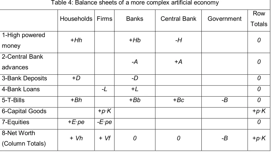
4.1.3 More Complex Financial Structures
What if the financial architecture discussed above is enriched to include high-powered
money, holdings of T-bills by families and central bank advances to banks? Table 4
below depicts the balance sheets of this more complex economy42.
Neglecting possible differences in taxation, the economy below differs from the
one discussed in the previous sections in three major ways. First, it implies a more
complex portfolio choice for households (who now have to choose among four instead of
two assets) and a potentially more complex determination of capitalist households’
income (given that the interest rates on deposits may differ from the interest rate on
T-bills). Second it implies a more complex role for banks, which now can hold money and
T-bills (being required by the central bank to hold a given minimum amount of
high-powered money). Third, it (trivially) changes the budget constraint of the government, for
now a part of the public debt is free of charge.
Table 4: Balance sheets of a more complex artificial economy
Households Firms Banks Central Bank Government Row
Totals
1-High powered
money +Hh +Hb -H 0
2-Central Bank
advances -A +A 0
3-Bank Deposits +D -D 0
4-Bank Loans -L +L 0
5-T-Bills +Bh +Bb +Bc -B 0
6-Capital Goods +p·K +p·K
7-Equities +E·pe -E·pe 0
8-Net Worth
(Column Totals) + Vh + Vf 0 0 -B +p·K
Keynes were well aware of this latter possibility is clear in Minsky (1975, p.119). See also Keynes (1937, p.668-9).
42
To see what is implied by the first two changes, consider the (Zezza and Dos
Santos, 2004) case in which:
pe·Ed = δ1·(Vh - Hhd); Dd = δ2·(Vh - Hhd) = Ds = D; Bhd =(1 - δ1 - δ2)·(Vh - Hhd) = Bh; Hhd = a1·u·p·K-1= Hh; and
Hbd = a2·D= Hb
It is now easy to see that the model now implies more complex specifications for both pe
and the SAVh and Vh functions. Beginning with the first, note that the new stock market equilibrium condition is:
pe·Ed = δ1·(Vh - Hhd) = pe·Es = pe·χ·K;
so that pe = (p·δ1·vh/χ) - [δ1·a1·u·p/χ·(1 + gi)]43.
Moreover, banks’ stock of loanable funds is reduced in this economy, for two basic
reasons: (i) households keep a part of their non-equity wealth in T-bills (so the amount of
bank deposits gets smaller); and (ii) banks are required to hold a fraction a2 of their total deposits D in high-powered money. So, the relevant equation for Bb becomes:
Bb = Max [0, (1-a2)·D – L], and, of course,
A = - Min [0, (1-a2)·D – L]44(i.e. A is one and the same as a negative Bb).
As a consequence, we have now two “regimes” in the model, i.e. one in which Bb is positive and another in which A is positive (presumably increasing the likelihood of the credit crunch regime45). If the interest rate on central bank advances and T-bills differ, each of these regimes will imply a different Fb equation and, therefore, different SAVh
and Vh equations. But given that A and Bb are straightforward functions of Vh, L and u, the model will still collapse to a buv system.
4.1.4 Inflation, Productivity and Distribution of Income
As mentioned before, the “fix-price” algebra above assumes implicitly that capacity
utilization does not reach its technical maximum. The model could easily incorporate a
43
As opposed to pe = (p·δ·vh/χ) in the simplified model.
44
The specification above implies either that the interest on T-bills is smaller than the interest on central bank’s advances or, if that is not the case, that the central bank monitors banks to ensure they do not get advances to finance purchases of T-bills.
45
“forced savings” regime (as discussed by Taylor, 1991, p.47), as well as a wide range of
(orthodox and heterodox) hypotheses about nominal wage, mark up and technical
progress dynamics.
More importantly from our perspective, a serious treatment of inflation would
require the model to be solved in “real” (i.e. deflated) terms. As discussed in section 1
above, this is straightforward for the flows but requires that the equations for all the
financial stocks assumed above are changed to include the “real capital gains” formulas
discussed in page 546. Finally, it is quite obvious that ceteris paribus inflation will hurt creditors (i.e. households and banks) and benefit debtors (i.e. firms and the government).
If large enough, it is likely to change the behavior of these sectors47, though it should now be obvious to the reader that these changes will not hurt the general (and now “real”) buv
structure, only make it more complex.
4.1.5 What if Vf = 0?
In this case the vh function (and the buv system) gets considerably simpler. Indeed, consolidating the balance sheets in table 1 above one gets:
Vh ≡ p·K + B,
or, equivalently,
(E27b) vh ≡ 1 + b.
But how can this new result be reconciled with our previous hypotheses?
Essentially, the answer to this question is that δ now gets endogenous, so the household
sector as a whole is supposed to always adjust their demand for equities to make sure it is
paying exactly what the firms are worth. To see this formally, note first that from the
firms’ balance sheet we have that:
p·K ≡ L + pe·E.
Plugging the firms’ loan demand (E16) in the identity above (and assuming χ = χ-1), one gets:
p·K ≡ (1 + i-1 - µ ·i-1)·L-1 + gi·p·K-1 - pe·gi·χ·K-1 – (1- µ)·(1-θ)·π·u·p·K-1+ pe·E; or, rearranging:
46
So that the stock equations are altered. As the required changes are both simple, tedious, and do not affect the gist of our argument, we will not discuss them in this text.
47
pe = (p /χ)·[1- l-1·(1- i-1 - µ ·i-1) + (1- µ)·(1-θ)·π·u]; so that
δ·Vh = δ·(p·K + B) = pe·E = (p /χ)·[1- l-1·(1- i-1 - µ ·i-1) + (1- µ)·π·u] ·E; or, after further rearranging:
δ = pe·E/ Vh = p·K·[1- l-1·(1- i-1 - µ ·i-1) + (1- µ)·π·u] / (p·K + B).
5 FINAL REMARKS
In the sections above we presented a simplified stock-flow consistent post-Keynesian
growth model and related it to the existing (structuralist and post-Keynesian)
liter-ature(s)48. We are well aware that the specific derivations above depend crucially on the simplifying assumptions we made. We note, however, that the general buv/blu structure discussed above appears to be robust to wide changes in the flow specifications and/or
financial architecture assumed—a point that, as far as we know, has not received enough
attention in the aforementioned literatures.
Of course, little in this paper is theoretically new. Borrowing words from Foley
and Sidrauski (1971, p. 6), our goal here was mostly to provide the reader with a rigorous
and didactic “exposition of an eclectic tradition that strikes us as particularly coherent
and logically convincing.” It is up to the reader to decide whether or not we have
succeeded.
48
References
Davidson, P. 1972. Money and the Real World, Armonk, New York: M.E. Sharpe
Dos Santos, C. 2004a. A Stock-Flow Consistent General Framework for Formal Minskyan
Analyses of Closed Economies, Working Paper No. 403, The Levy Economics Institute of
Bard College, Annandale-on-Hudson, New York. Forthcoming in the Journal of
Post-Keynesian Economics
__________ 2004b. Keynesian Theorizing During Hard Times: Stock-Flow Consistent Models as
an Unexplored “Frontier” of Keynesian Macroeconomics. Working Paper No. 408, Levy
Economics Institute of Bard College, Annandale-on-Hudson, New York. Forthcoming in
the Cambridge Journal of Economics
Delli Gatti, D., Gallegati, M. and Minsky, H. 1994. Financial Institutions, Economic Policy and
the Dynamic Behavior of the Economy, Working Paper No. 126, Levy Economics
Institute of Bard College, Annandale-on-Hudson, New York.
Foley, D. and Sidrauski, M. 1971. Monetary and Fiscal Policy in a Growing Economy. London:
McMillan
Foley, D. and Taylor, L. 2004. A Heterodox Growth and Distribution Model. Paper presented in
the “Growth and Distribution Conference,” University of Pisa, June 16–19
Franke, R and Semmler, W. 1989 Debt Dynamics of Firms, Stability and Cycles in a Dynamical
Macroeconomic Growth Model. In Semmler, W (ed.) Financial Dynamics and the
Business Cycles: New Perspectives, Armonk, 18-37, New York: ME Sharpe
Godley, W. 1996. Money, Income and Distribution: an Integrated Approach, Working Paper No.
167, The Levy Economics Institute of Bard College, Annandale-on-Hudson, New York.
_______ 1999. Money and Credit in a Keynesian Model of Income Determination, Cambridge
Journal of Economics, Vol. 23, No. 4, July, 393-411
Godley, W. and Cripps, F. 1983. Macroeconomics, Oxford: Oxford University Press
Graziani, A. 2003. The Monetary Theory of Production, Cambridge: Cambridge University Press
Keynes, J.M. 1997 [1936]. The General Theory of Employment, Interest and Money, Amherst,
NY: Prometheus Books
_________ 1937. The "Ex-Ante" Theory of the Rate of Interest, The Economic Journal, Vol. 47,
No. 188, December, pp. 663-669
Lavoie, M. and Godley, W. 2001-2002. Kaleckian Growth Models in a Stock and Flow Monetary
Framework: A Kaldorian View. Journal of Post Keynesian Economics, Vol.24, No. 2,
277-311, Winter
Marglin. S. and Bhaduri, A. 1990. Unemployment and the Real Wage: The Economic Basis for
Contesting Political Ideologies, Cambridge Journal of Economics, Vol. 14, No .4,
December, 375-393
Minsky, H. 1975. John Maynard Keynes, New York: Columbia University Press
________ 1982. Can it Happen Again? Armonk, New York: M.E. Sharpe
________ 1986. Stabilizing an Unstable Economy, New Haven, CT: Yale University Press, 1986
Modigliani, F. and Miller, M. 1958, “The Cost of Capital, Corporation Finance and the Theory of
Investment.” American Economic Review, Vol.48, No.3, June, 261-297
Moudud, J. 1998. Endogenous Growth Cycles and Money in an Open Economy: A Social
Accounting Matrix Approach. Unpublished PhD Thesis, New School for Social Research,
NY, 1998
Palley, T. 1996. Post Keynesian Macroeconomics, New York: St. Martin’s Press
Shaikh, A. 1989. A Dynamic Approach to the Theory of Effective Demand, Working Paper No.
19, Levy Economics Institute of Bard College, Annandale-on-Hudson, NY.
Skott, P. 1989. Conflict and Effective Demand in Economic Growth, Cambridge: Cambridge
University Press
Stiglitz, J. and Greenwald, B. 2003. Towards a New Paradigm in Monetary Economics,
Cambridge: Cambridge University Press
Taylor, L. 1991. Income Distribution, Inflation and Growth, Cambridge, Massachusetts: MIT
Press
________2004. Reconstructing Macroeconomics, Cambridge, Massachusetts: Harvard University
Press
Taylor, L. and O’Connel, S. 1985. A Minsky Crisis. Quarterly Journal of Economics, Vol.100,
Supplement, 871-885
Tobin, J. 1980. Asset Accumulation and Economic Activity,Chicago, IL: University of Chicago
Press
_______ 1982. Money and the Macroeconomic Process. Journal of Money, Credit and Banking,
Tobin, J. and Golub, S. 1998. Money, Credit and Capital. New York: Irwin McGraw Hill
Walsh, C. 1998. Monetary Theory and Policy. Cambridge, Massachusetts: MIT Press
Zezza, G. and Dos Santos, C.H. 2004. The Role of Monetary Policy in Post-Keynesian
Stock-Flow Consistent Macroeconomic Growth Models: Preliminary Results. In Lavoie, M. and
Seccareccia. M. (eds.), Central Banking in the Modern World: Alternative Perspectives,
APPENDIX
As the u curve was derived earlier in the text, we begin by deriving the b and vh curves.
A.1 – The b curve
From (E19) and (E24) we have that:
(A.1.1) B = (1 + ib-1)·B-1 + γ·p·K-1 - θ·p·X; or, dividing everything by p·K-1,
(A.1.2) b·(1 + gi) = (1 + ib-1)·b-1 + γ - θ·u, where:
b-1 = B-1/(p·K-1), and b = B/(p·K).
It is now straightforward to see that:
(E26) b = [b-1·(1+ib-1) +γ - θ·u ] / (1 + gi)49.
A.2 –The vh curve
From (E10), (E12) and (E21) we have that:
(A.2.1) Vh = (1 - a)·Vh-1 + µ ·(1-θ)·π·u·p·K-1 + (1- µ)·i-1·L-1+ ib-1·B-1 +∆pe·E-1;
Moreover, from (E11) and (E15) (and assuming that δ-1 = δ and χ = χ-1) we have that: (A.2.2.) ∆pe·E-1 = δ·Vh/(1 + gi) - δ·Vh-1;
and from the balance sheets of banks and (E8) we know that
(A.2.3.) L-1 = (1 - δ)·Vh-1 - B-1;
So, replacing (A.2.2) and (A.2.3) in (A.2.1) and rearranging, we get:
(A.2.4)Vh=[1-a-δ+(1- δ)·(1- µ)·i-1]·Vh-1+ µ ·(1-θ)·π·u·p·K-1+[ib-1 -(1- µ)·i-1]·B-1 +δ ·Vh/(1+gi) or, dividing both sides by p·K-1,
(A.2.5)Vh/p·K-1 = ψ1·vh-1+ µ ·(1-θ)·π·u + ψ2·b-1 +δ ·vh; where:
ψ1 = [1- a - δ + (1- µ)·(1 - δ)·i-1]; ψ2 = ib-1 - (1 - µ) ·i-1;
b-1 = B-1/(p·K-1); vh-1 = Vh-1/(p·K-1); and
49
vh= Vh/(p·K).
As (by definition) Vh/p·K-1 = vh·(1+gi), it is now straightforward to show that: (E27) vh = [ψ1·vh-1+ µ ·(1-θ)·π·u + ψ2·b-1] /·(1+gi – δ)50.
A.3 – The slope of the b and vh curves
All one needs to do to get the slopes of the curves above (depicted in section 3.1.1) is to
derive them with respect to u. It is intuitively clear, however, that ∂b/∂u < 0 for increases in the economic activity generates increases in investment (and therefore capital growth)
and in tax revenues, and both factors contribute to a smaller b. It so happens that ∂vh/∂u
is also negative for a wide range of parameters and initial conditions. Indeed, increases in
real activity have only a relatively modest positive impact on the stock of households’
wealth (through its impact on the distributed profits of firms and, therefore, on
households’ income and saving) and affect the growth of the capital stock importantly
(therefore affecting vh = Vh/p·K negatively)51. Finally, given that b and vh completely determine l, it is clear that ∂l/∂u also tends to be negative.
A.4 – The steady-state solution of the buv system
All one needs to do to get the steady state solution of the buv system is to solve it
assuming that vh = vh-1 and b = b-1. It is then relatively easy to show that the characteristic equation of the system is cubic (what is unsurprising given the
non-linearites in the buv system), potentially allowing for multiple (i.e. up to 3) “long run” equilibria. In the numeric example discussed in the text, however, two of the roots of the
system were imaginary, so the steady-state solution depicted in section 3.2 was the only
real one.
50
So that a necessary condition for the stability of the buv system is that ψ1/·(1+gi – δ) < 1, or equivalently that g >(1- µ)·(1 - δ)·i-1- a.
51
This point can be seen formally. Indeed, it is easy to prove that ∂vh/∂u<0 when vh >µ·(1-θ)·π/(α·π+ β).