A SIMPLIFIED, ‘BENCHMARK’, STOCK-FLOW CONSISTENT
POST-KEYNESIAN GROWTH MODEL
Claudio H. Dos Santos and Gennaro Zezza*
Institute for Applied Economic Research, Ministry of Planning of Brazil
and Levy Economics Institute of Bard College, and University of Cassino,
Italy and Levy Economics Institute of Bard College
(January 2006, revised August 2007)
ABSTRACT
Despite being arguably one of the most active areas of research in heterodox macroeconomics, the study of the dynamic properties of stock-flow consistent (SFC) growth models of financially sophis-ticated economies is still in its first steps. This paper attempts to offer a contribution to this line of research by presenting a simplified SFC Post-Keynesian growth model with well-defined dynamic properties and using it to shed light on the merits and limitations of the current heterodox SFC literature.
It will be the objective of the historical model developed below to provide a simple analysis of capital accumulation by blending the stock and flow elements in the demand and supply of (i) real capital, (ii) money, and (iii) securities (. . .) with the more familiar concepts (. . .) of effective demand developed in the General Theory. Within such a framework it is possible to provide more perspec-tive on the interplay among organized security exchanges, corporate financing policy, investment underwriters and the banking system in channeling the finan-cial funds necessary for capital accumulation. Regrettably this is an analysis which is virtually ignored in most ‘analytical’ Post-Keynesian models. (Davidson, 1972, p. 31)
* This paper is a new version of Dos Santos and Zezza (2005), which has been substantially revised. We would like to thank Duncan Foley, Wynne Godley, Marc Lavoie, Anwar Shaikh, Peter Skott, Lance Taylor and two anonymous referees for commenting on previous versions of this paper. The remaining errors in the text are all ours. Derivation of some results in the text, along with a full list of symbols and an Excel file to compute numerical simulations, can be downloaded from http://gennaro.zezza.it/papers/zds2007/.
1. INTRODUCTION
In recent years, a significant number of ‘stock-flow consistent’ (SFC)
Post-Keynesian growth models and articles have appeared in the literature,
1making it one of the most active areas of research in Post-Keynesian
mac-roeconomics. Yet, it is fair to say that most of the discussion so far has been
phrased in terms of relatively complex, and often exploratory,
(computer-simulated) models and that this has prevented the dissemination of the main
insights of this literature to broader audiences.
2This paper attempts to ease
this problem by presenting a simplified (and, we hope, representative)
Post-Keynesian SFC growth model that, in our view, sheds considerable light on
the merits and limitations of existing (and usually more complex) heterodox
SFC models, and could conceivably be used as a ‘benchmark’ to facilitate
discussion among authors of these models and authors in various other
Post-Keynesian and related traditions.
Most of the appeal of Post-Keynesian SFC models, as well as the
difficul-ties associated with them, stems from two basic features of these constructs,
i.e. the facts that: (1) they are, in a sense to be explained below, ‘intrinsically
dynamic’ (Turnovsky, 1977, p. 3), and (2) they model financial markets and
real–financial interactions explicitly. Therefore, the relative merits of the SFC
literature are more easily appreciated in the context of the discussion of how
Post-Keynesians have conceptualized dynamic trajectories of real economies
in historical time and how these are affected by financial markets’ behavior.
Beginning with the latter issue, we have noted elsewhere
3that there is a
widespread consensus, among prominent Keynesians of all persuasions,
4about the role played by financial markets, notably stock and credit markets,
in the determination of the demand price for capital goods (and, hence, of
investment demand, via some version of ‘Tobin’s
q’) and in the financing of
investment decisions. The role played by banks in the financing of investment
is acknowledged by Keynes, for example, in the famous passage in which he
notes that ‘the investment market can become congested through a
short-age of cash’ (Keynes, 1937, p. 669). More emphatically, Minsky argues that
1See Taylor (1985), Lavoie and Godley (2001–2), Foley and Taylor (2004), Zezza and Dos Santos (2004) and Dos Santos (2005, 2006), among many others. The current literature builds on the seminal work of, among others, Tobin (1980, 1982) and Godley and Cripps (1983). See Dos Santos (2006) for a detailed discussion of these authors’ contributions and Dos Santos (2005) for a discussion of the related ‘Minskyan’ literature of the 1980s–90s. The seminal work of Moudud (1998) with SFC models in the tradition of classical economists is also worth mentioning. A recent major contribution has been provided by Godley and Lavoie (2007).
2A notable exception is the theoretical models in Taylor (2004). 3Dos Santos (2006).
investment theories that neglect the financing needs of investing firms
amount to ‘palpable nonsense’ (Minsky, 1986, p. 188).
This consensus is extensible to the idea that asset prices are determined by
the portfolio decisions of the various economic agents, being only marginally
affected—if at all—by current saving flows. In the words of Davidson, ‘in the
real world, new issues and household savings are trifling elements in the
securities markets (. . .). Any discrepancy between (. . .) [new issues] and (. . .)
[the “flow” demand for new securities] is likely to be swamped by the eddies
of speculative movements by the whole body of wealth-holders who are
constantly sifting and shifting their portfolio composition’ (Davidson, 1972,
p. 336).
In other words, most Post-Keynesians would agree that the size and the
desired composition of the balance sheets of the various institutional sectors
(i.e. households, firms, banks, and the government, in a closed economy)
determine (short period) ‘equilibrium’ asset prices which, in turn, crucially
affect ‘real [macroeconomic] variables’.
Few Post-Keynesians would disagree also that ‘Keynes’s formal analysis
dealt only with a period of time sufficiently brief (Marshall’s short period of
a few months to a year) for the changes taking place in productive capacity
over that interval, as a result of net investment, to be negligible relative to the
total inherited productive capacity’ (Asimakopulos, 1991, p. xvi).
Accord-ingly, many Post-Keynesians have argued that extending Keynes’s analysis
to ‘the long period’ involves ‘linking adjacent short periods, which have
different productive capacities, and allowing for the interdependence of
changes in the factors that determine the values of output and employment in
the short period[s]’ (Asimakopulos, 1991).
Essentially the same view was espoused by Joan Robinson (1956,
pp. 180–181) and by Michael Kalecki, in an often quoted passage in which he
notes that ‘the long run trend is but a slowly changing component of a chain
of short-period situations. It has no independent entity’ (Kalecki, 1971,
p. 165). Not all Post-Keynesians agree with it, though. Skott (1989, p. 43),
for example, criticizes this Asimakopulos–Kalecki–Robinson view on the
grounds that, when coupled with the usual Keynesian assumption
5that firms’
short-period expectations are roughly correct, it implies—given constant
animal spirits—that the economy is always in long-period equilibrium, as
defined by Keynes in chapter 5 of the General Theory. While this last point
is certainly correct, we do not see it as a bad thing. In fact, we argue in section
3 that a careful analysis of Keynes’ long-period equilibrium is much more
useful than conventional wisdom would make us believe.
It so happens that the careful modeling of stock-flow relations provides a
natural and rigorous link between ‘adjacent short periods’. In particular, it
makes sure that the balance sheet implications of saving and investment flows
and capital gains and losses in any given short period are fully taken into
consideration by economic agents in the beginning of the next short period.
This, in turn, is crucial in Post-Keynesian models, for if one assumes that
asset prices are determined by the portfolio choices of the various economic
agents, one must also acknowledge that dynamically miscalculated balance
sheets would imply increasingly wrong conclusions about financial markets’
behavior.
In sum, and despite its somewhat discouraging algebraic form, the broader
goal of current SFC literature is very similar to the one stated by Davidson
in the passage above.
6In fact, most of the (simple, though admittedly
tedious) algebra below is meant only to make sure we are getting the
dynam-ics of the balance sheets right and, therefore, approaching Davidson’s
problem from a more explicitly dynamic standpoint.
The structural and behavioral hypotheses of our model are presented in
section 2 below, while section 3 discusses (the meaning of) its short- and
long-period equilibria. Section 4 briefly discusses how the model presented
here relates to the broader heterodox SFC literature. Section 5 concludes.
2. THE MODEL IN THE SHORT RUN
2.1
Structural hypotheses and their system-wide and dynamic implications
The economy assumed here has households, firms (which produce a single
good, with price
p), banks and a government sector. The aggregated assets
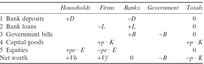
and liabilities of these institutional sectors are presented in table 1.
Table 1 summarizes several theoretical assumptions. First, and for
simpli-fication purposes only, we assume a ‘pure credit economy’, i.e. that all
transactions are paid with bank checks. This hypothesis is used only to
simplify the algebra and can easily be relaxed without changing the essence of
the argument. It is important to notice, however, that the financial structure
assumed above rules out financial disintermediation (and therefore systemic
bank crises) by hypothesis. Therefore, allowing for cash holdings will be
necessary in more realistic settings.
Households are assumed not to get bank loans and to keep their wealth
only in the form of bank deposits and equities. The reason why households
do not care to buy government bills is that banks are assumed to remunerate
deposits at the same rate the government remunerates its bills.
7Banks are
also assumed to: (1) always accept government bills as means of payment for
government deficits, (2) not pay taxes, and (3) to distribute all its profits, so
its net worth is equal to zero.
We will thus be working with the conventional case in which the
govern-ment is in debt (B
>
0), noting that not too long ago—in the Clinton years, to
be precise—analysts were discussing the consequences of the US paying all its
debt. A negative
B, i.e. a positive government net worth, can be interpreted
in this model as ‘net government advances’ to banks. We are also simplifying
away banks’ and government’s investment in fixed capital, as well as their
intermediary consumption (wages, etc.). These assumptions are made only
to allow for simpler mathematical expressions for household income and
aggregate investment.
Firms are assumed to finance their investment using loans, equity emission
and retained profits.
8Moreover, the Modigliani–Miller (1958) theorem does
not hold in this economy, so the specific way firms choose (or find) to finance
themselves matters. As it has been pointed out, ‘the greater the ratio of equity
to debt financing the greater the chance that the firm will be a hedge financing
unit’ (Delli Gatti
et al., 1994, p. 13). This ‘Minskyan’ point is, of course, lost
7 So that lending to firms is banks’ only source of profits. According to Stiglitz and Greenwald (2003, p. 43), a banking sector with these characteristics ‘is not too different from what may emerge in the fairly near future in the USA’. In any case, this hypothesis allows us to simplify the portfolio choice of households considerably. More detailed treatments, such as the ones in Tobin (1980) or Lavoie and Godley (2001–2), can easily be introduced, though only at the cost of making the algebra considerably heavier.
8 As in Skott (1989) and Godley and Lavoie (2007), for example.
Table 1. Aggregate balance sheets of the institutional sectors
Households
Firms
Banks
Government
Totals
1 Bank deposits
+
D
-
D
0
2 Bank loans
-
L
+
L
0
3 Government bills
+
B
-
B
0
4 Capital goods
+
p
·
K
+
p
·
K
5 Equities
+
pe
·
E
-
pe
·
E
0
Net worth
+
Vh
+
Vf
0
-
B
-
p
·
K
in a Modigliani–Miller world, as in models in which firms issue only one form
of debt.
The ‘current flows’ associated with the stocks above are described in
table 2. As such, it represents very intuitive phenomena. Households in
vir-tually all capitalist economies receive income in form of wages, interest on
deposits, and distributed profits of banks and firms and use it to buy
con-sumption goods, pay taxes and save, as depicted in the households’ column
of table 2. We simplify away household debt and housing investment. The
government, in turn, receives money from taxes and uses it to buy goods from
firms and pay interest on its lagged stock of debt, while firms use sales receipts
to pay wages, taxes, interest on their lagged stock of loans and dividends,
retaining the rest to help finance investment. Finally, banks receive money
from their loans to firms and holdings of government bills and use it to pay
interest on households’ deposits and dividends.
In a ‘closed system’ such as ours every money flow has to ‘come from
somewhere and go somewhere’ (Godley, 1999, p. 394), and this shows up in
the fact that all row totals of table 2 are zero. Note also that firms’ investment
expenditures in physical capital imply a change in their financial or capital
assets and, therefore, are ‘capital’ transactions. As such they (re)appear in
table 3. The reason they are included in table 2 is to stress the idea that firms
buy their capital goods from themselves—an obvious feature of the real
world, though a slightly odd assumption in our ‘one good economy’.
While it is true that beginning-of-period stocks necessarily affect income
flows, as depicted in table 2, it is also true that saving flows and capital gains
necessarily affect end-of-period stocks, which, in turn, will affect next
peri-od’s income flows. This ‘intrinsic SFC dynamics’ is shown in table 3. Note
that fluctuations in the price of the single good produced in the economy (for
firms) and in the market value of equities (for firms and households) are the
only sources of nominal capital gains and losses in this economy.
Given the hypotheses above, households’ saving necessarily implies
changes in their holdings of bank deposits and/or stocks, while government
deficits are necessarily financed with the emission of government bills, and
investment is necessarily financed by a combination of retained earnings,
equity emissions and bank loans. As emphasized by Godley (1999), banks
play a crucial role in making sure these inter-related balance sheet changes
are mutually consistent.
9Table 2. ‘Current’ transactions in our artificial economy
Households
Firms
Government
Banks
Totals
Current
Capital
1 Consumption
-
C
+
C
0
2 Government expenditure
+
G
-
G
0
3 Investment in fixed
K
+
p
·
D
K
-
p
·
D
K
0
4 Accounting memo: ‘Final’ sales at market prices
=
p
·
X
≡
C
+
G
+
p
·
D
K
≡
W
+
FT
≡
Y
5 Wages
+
W
-
W
0
6 Taxes
-
Tw
-
Tf
+
T
0
7 Interest on loans
-
il
t-1·
L
t-1+
il
t-1·
L
t-10
8 Interest on bills
-
ib
t-1·
B
t-1+
ib
t-1·
B
t-10
9 Interest on deposits
+
ib
t-1·
D
t-1-
ib
t-1·
D
t-10
10 Dividends
+
Fd
+
Fb
-
Fd
-
Fb
0
11 Column totals
SAVh
Fu
-
p
·
D
K
SAVg
0
0
Note: A (+) sign before a variable denotes a receipt, while a (-) sign denotes a payment.
Simplified
SFC
Post-Keynesian
Growth
Model
The
Authors
compilation
©
2008
Blackwell
Publishing
Table 3. Flows of funds in our artificial economy
Households
Firms
Government
Banks
Totals
1 Current saving
+
SAVh
+
Fu
+
SAVg
0
+
SAV
2
D
Bank deposits
-D
D
+D
D
0
3
D
Loans
-D
L
-D
L
0
4
D
Government bills
-D
B
+D
B
0
5
D
Capital
-
p
·
D
K
-
p
·
D
K
6
D
Equities
-
pe
·
D
E
+
pe
·
D
E
0
Totals
0
0
0
0
0
D
Net worth (
accounting
memo
)
D
Vh
=
SAVh
+
D
pe
·
E
t-1D
Vf
=
Fu
+ D
p
·
K
t-1-D
pe
·
E
t-1+
SAVg
0
SAV
+ D
p
·
K
t-1=
+
p
·
D
K
+ D
p
·
K
t-1Note: Positive figures denote sources of funds, while negative ones denote uses of funds.
Claudio
H.
Dos
Santos
and
Gennaro
Zezza
The
Authors
compilation
©
2008
Blackwell
Publishing
We finish this section reminding the reader that all accounts presented so
far were phrased in nominal terms. All stocks and flows in tables 1 and 2 have
straightforward ‘real’ counterparts given by their nominal value divided by
p
(the price of the single good produced in the economy), while the ‘real’ capital
gains in equities are given by
Δ
pe E
t⋅
t−
Δ
p pe
t⋅
t⋅
E
tp
tp
t(
−1 −1 −1 −1)
(1)
and the ‘real’ capital gains in any other financial asset
Z
are given by
10−
Δ
p
t⋅
(
Z
t−1p
t−1)
p
t(2)
We believe that the artificial economy described above—though not
nec-essarily its accounting details—is quite familiar to most macroeconomists in
the broad Post-Keynesian tradition. In order to keep things simple, we will
try as much as possible to ‘close’ it with (dynamic versions of) equally
familiar Keynes/Kalecki hypotheses. Of course, given that modeling
‘econo-mies as a whole’ from a financially sophisticated Post-Keynesian standpoint
implies making a relatively large number of simplifying assumptions about
both the behavior and the composition of the various relevant sectors of the
economy, very few people will agree with everything in our model. We do
hope, however, that a sufficient number of Post-Keynesians will deem it
representative enough of their own views to deserve attention or, at least, will
find illuminating to phrase their dissenting views as alternative structural
or behavioral hypotheses about the obviously simplified artificial economy
discussed above. If this turns out to be the case, we will consider ourselves
successful in our main goal of providing a ‘benchmark’ model in order to
facilitate discussion among economists of the various Post-Keynesian and
related traditions.
2.2
A horizontal aggregate supply curve
Following Taylor (1991, ch. 2), we assume that
p
t=
w
t⋅ ⋅ +
λ
t(
1
τ
)
(3)
where
p
=
price level,
w
=
money wage per unit of labor,
l
=
labor–output
ratio,
t
=
mark-up rate.
11From (1) it is easy to prove that the (gross, before
tax) profit share on total income (
p
) is given by
10 Given that ours is a ‘one good’ economy, the real value of physical capital is not affected by inflation.
π
τ
so that the (before tax) wage share on total income is
1
1
We assume here also that the nominal wage rate, the technology and the
income distribution of the economy are exogenous, so all lower-case
vari-ables above are constant, and therefore the aggregate supply of the model is
horizontal. In other words, we work here with a fix-price model in the sense
of Hicks (1965, p. 77–78). All these assumptions can be relaxed, of course,
provided one is willing to pay the price of increased analytical complexity. In
particular, they allow us to avoid here unnecessary complications related to
inflation accounting.
2.3
Aggregate demand
2.3.1
A ‘Kaleckian SFC’ consumption function
The simplifying hypothesis here is that wages after taxes are entirely spent,
while ‘capitalist households’—receiving distributed profits from firms and
banks—spend a fraction of their lagged wealth—as opposed to their current
income, as in Kalecki.
12The presence of household wealth in the
consump-tion funcconsump-tion is, of course, compatible with Modigliani and Brumberg (1954)
seminal work. Formally,
C
t=
W
t−
Tw
t+ ⋅
a Vh
t−1=
W
t⋅ −
(
1
θ
)
+ ⋅
a Vh
t−1(7)
where
q
is the income tax rate and
a
is a fixed parameter. Following Taylor,
we normalize the expression above by the (lagged) value of the stock of
capital
13to get
12 We have analyzed elsewhere (Zezza and Dos Santos, 2006) the relationship between income distribution and growth in this class of models, and we chose to adopt a simple specification in the present version.
C
t(
p K
t⋅
t−1)
= −
(
1
π
)
⋅ −
(
1
θ
)
⋅ + ⋅
u
ta vh
t−1(8)
where
u
t=
X
t/K
t-1and
vh
t=
Vh
t/(p
t·
K
t).
14Needless to say, equation (8) is
compatible with the conventional simplified Keynesian short-period
specifi-cation (C
t=
C
0+
c
·
Yd
t), provided one makes
C
0=
a
·
Vh
t-1and
c
=
1
-
p
.
2.3.2
A ‘Neo-Kaleckian’ investment function
The simplest version of the model presented here uses Taylor’s (1991, ch. 5)
‘structuralist’ investment function, which, in turn, is an extension of the one
used by Marglin and Bhaduri (1990) and a special case of the one used in
Lavoie and Godley (2001–2). Given that investment functions are a topic of
intense controversy in heterodox macroeconomics—see, for example, Lavoie
et al. (2004)—it would be interesting to study the implications of ‘Harrodian’
(or ‘Classical’) specifications in which investment demand gradually adjusts
to stabilize capacity utilization—as proposed, among others, by Shaikh
(1989) and Skott (1989). Section 4 discusses this issue in greater detail,
although space considerations have forced us to postpone a complete
treat-ment to another occasion. Our current specification follows the broad
structuralist literature in assuming, for simplification purposes, that the
output–capital ratio is a good measure of capacity utilization. In symbols, we
have
g
t=
g
0+
(
α π β
⋅ +
)
⋅ − ⋅
u
tθ
1il
t(9)
where
g
t= D
K
t/K
t-1,
il
is the (real) interest rate on loans, and
g
0,
a
,
b
and
q
1are
exogenous parameters measuring the state of long-term expectations (g
0), the
strength of the ‘accelerator’ effect (
a
and
b
) and the sensibility of aggregate
investment to increases in the interest rate on bank loans (
q
1). In section 4.2
we discuss what happens when one modifies this investment function along
the lines suggested by Lavoie and Godley (2001–2).
requirements are reasonably complex in continuous time, and no proportional insight appears to be added, we work here in discrete time and assume—as Keynes—that the stock of capital available in any given ‘short period’ is pre-determined, i.e. that investment does not translate into capital instantaneously. We thus normalize all flows by the opening stock of capital, and stocks by the current stock of capital.
2.3.3
The ‘u’ curve
Assuming that both
g
t=
G
t/(p
t·
K
t-1) and
il
are given by policy, the
‘short-period’ goods’ market equilibrium condition is given by
p X
t⋅
t=
W
t⋅ −
(
1
θ
)
+ ⋅
a Vh
t−1+
[
g
0+
(
α π β
⋅ +
)
⋅ − ⋅ +
u
tθ
1il
tγ
t]⋅ ⋅
p K
t t−1(10)
or, after trivial algebraic manipulations,
u
t=
ψ
1⋅
A il
( )
t+
ψ
1⋅ ⋅
a vh
t−1(11)
where
ψ
1=
1 1
[
− −
(
1
π
)
⋅ −
(
1
θ
)
−
α
1]
(12)
α
1= ⋅ +
α π β
(13)
A il
( )
t=
g
0− ⋅ +
θ
1il
tγ
t(14)
Equation (11) is essentially the normalized ‘IS’ curve of the model. Notice
that, as for a textbook IS curve, the level of economic activity is determined
by a multiplier
y
1, times autonomous demand
A, which here is given by the
normalized government expenditure
g
and autonomous growth in investment
g
0, plus additional effects from the interest rate and the opening stock of
wealth.
In fact, the ‘short-period’ equilibrium of the model, represented in figure 1,
has a straightforward ‘IS-LM’ (of sorts) representation, which implies that
‘short-period’ comparative static exercises can be done quite simply. Note
finally that, the (temporary, goods’ market) equilibrium above only makes
u u*
i
i*
Capacity barrier
economic sense if the sum of the propensity to consume out of current income
(i.e. (1
-
p
) · (1
-
q
)) and the ‘accelerator’ effect (i.e.
a
1=
a
·
p
+
b
) is smaller
than one. The (short-period) consequences of having the income distribution
impacting both the multiplier and the accelerator of the economy were
exam-ined in the classic paper by Marglin and Bhaduri (1990).
2.4
Financial markets
2.4.1
Financial behavior of households
The two crucial hypotheses here are that: (1) households make no
expecta-tion mistakes concerning the value of
Vh, and (2) the share
d
of equity (and,
of course, the share 1
-
d
of deposits) on total household wealth depends
negatively (positively) on
ib
and positively (negatively) on the expectational
parameter
r
.
15Formally,
pe E
t⋅
td= ⋅
δ
Vh
t(15)
D
td= −
(
1
δ
)
⋅
Vh
t(16)
δ
= − +
ib
ρ
(17)
where
r
is assumed to be constant in this simplified ‘closure’.
16The simplified
specification above follows Keynes in assuming that the demand for equities
‘. . . is established as the outcome of the of the mass psychology of a large
number of ignorant individuals (. . .)’ and, therefore, is ‘liable to change
violently as the result of a sudden fluctuation in opinion due to factors that
do not really much make difference to the prospective yield (. . .)’ (Keynes,
1936, p. 154). The value of
Vh, on the other hand, is given by the households’
budget constraint (see table 3).
Vh
t≡
Vh
t−1+
SAVh
t+
Δ
pe E
t⋅
t−1(18)
while from table 2 and equation (7) it is easy to see that
SAVh
t= +
ib
t−1⋅
D
t−1+
Fd
t+
Fb
t− ⋅
a Vh
t−1(19)
15 Note that, as discussed in more detail in section 3, the inclusion of expectation errors—say, along the lines of Godley (1999)—would imply the inclusion of hypotheses about how agents react to them, making the model ‘heavier’.
so that:
Vh
t= −
(
1
a Vh
)
⋅
t−1+
ib
t−1⋅
D
t−1+
Fd
t+
Fb
t+
Δ
pe E
t⋅
t−1(20)
2.4.2
Financial behavior of firms
For simplicity, we assume that firms keep a fixed
E/K
rate
c
and distribute a
fixed share
m
of its (after-tax, net of interest payments) profits.
17We thus have
E
tK
K
g
And, as the price of equity
pe
is supposed to clear the market, we have also
that
Firms’ demand for bank loans, in turn, can be obtained from their budget
constraint (see table 3). Indeed, from
Δ
L
t≡ ⋅
p
tΔ
K
t−
pe
t⋅
Δ
E
t−
Fu
t(26)
it is easy to see that, by replacing equations (21) and (23) in (26),
L
il
L
g p
pe g
2.4.3
Financial behavior of banks and the government
For simplicity, banks are assumed here—a la
Lavoie and Godley (2001–2)
and Godley and Lavoie (2007)—to provide loans as demanded by firms. In
fact, banks’ behavior is essentially passive in the simplified model discussed
here, for we also assume that: (1) banks always accept deposits from
house-holds and bills from the government, (2) banks distribute whatever profits
they make,
18and (3) the interest rate on loans is a fixed mark-up on the
interest rate on government bills. Formally,
L
tL
L
st d
t
=
=
(28)
D
tD
D
st d
t
=
=
(29)
B
tB
B
st d
t
=
=
(30)
il
t= +
(
1
τ
b)
⋅
ib
t(31)
Fb
t=
il
t−1⋅
L
t−1+
ib
t−1⋅
B
t−1−
ib
t−1⋅
D
t−1(32)
The government, in turn, is assumed to choose: (1) the interest rate on its bills
(ib), (2) its taxes (as a proportion
q
of wages and gross profits), and (3) its
purchases of goods (as a proportion
g
of the opening stock of capital), while
the supply of government bills is determined (as a residual) by its budget
constraint:
G
t= ⋅ ⋅
γ
tp K
t t−1(33)
T
t=
Tw
t+
Tf
t= ⋅
θ
W
t+ ⋅
θ
(
p X
t⋅
t−
W
t)
= ⋅ ⋅
θ
p X
t t(34)
B
ts= +
(
1
ib
t−1)
⋅
B
t−1+ ⋅ ⋅
γ
p K
t t−1− ⋅ ⋅
θ
p X
t t(35)
3. COMPLETE ‘TEMPORARY’ AND ‘STEADY-STATE’ SOLUTIONS
As noted above, the SFC approach allows for a natural integration of ‘short’
and ‘long’ periods. In particular, both Keynesian notions of ‘long-period
equilibrium’ and ‘long run’ acquire a precise sense in a SFC context, the
former being the steady-state equilibrium of the stock-flow system (assuming
that all parameters remain constant through the adjustment process), and the
latter being the more realist notion of a path-dependent sequence of ‘short
periods’ in which the parameters are subject to sudden and unpredictable
changes. These concepts are discussed in more detail in section 3.3. Before we
do that, however, we need discuss the characteristics of the ‘short-period’ (or
‘temporary’) equilibrium of the model.
3.1
The ‘short-period’ equilibrium
In any given (beginning of) period, the stocks of the economy are given,
inherited from history. Under these hypotheses, and given distribution
and policy parameters, we saw in section 2.3.3 that the (normalized) level
of economic activity—assuming that the economy is below full capacity
utilization—is given by
19u
t=
ψ
1⋅
A ib
( )
t+
ψ
1⋅ ⋅
a vh
t−1(11
′
)
But (demand-driven) economic activity is hardly the only variable
deter-mined in any given ‘short period’. As noted above, the balance sheet
impli-cations of each period’s sectoral income and expenditure flows and portfolio
decisions are also (dynamically) crucial. Here the hypothesis that banks have
zero net worth proves to be convenient, for it implies that the stock of bank
loans (L) is determined by the stock of government debt (B) and by the stock
of household wealth (Vh). Specifically, given that
L
+
B
≡
D
(from table 1)
and
D
=
(1
-
d
) ·
Vh
from equations (16) and (29), we have that
L
t= −
(
1
δ
)
⋅
Vh
t−
B
t(36)
It so happens that all other endogenous stocks and flows of the model are
easily determined from
u
and (the normalized values of)
B
and
Vh.
Accord-ingly, the remaining of this section will be spent computing the latter
variables. The case of
B
is the simplest one. From equations (30) and (35) we
have that
B
t=
B
t−1⋅ +
(
1
ib
t−1)
+ ⋅ ⋅
γ
tp K
t t−1− ⋅ ⋅
θ
p X
t t(37)
i.e. that the end-of-period government debt is given by beginning-of-period
government debt plus the government’s interest payments (ib
t-1·
B
t-1) and
purchases of public goods (
g
t·
p
t·
K
t-1) minus its tax revenues (
q
·
p
t·
X
t).
Now, dividing the equation above by
p
t·
K
t-1and rearranging, we get
b
t=
[
b
t−1⋅ +
(
1
ib
t−1)
+
γ
t− ⋅
θ
u
t]
(
1
+
g
t)
(38)
19 We now use (31) into (14) to get autonomous demand relative to the interest rate on bills:
where,
b
t=
B
t/(p
t·
K
t).
20In words, the
normalized
value of the government
debt will increase (decrease) when the level of government debt increases
faster (slower) than the value of the stock of capital.
To calculate the normalized value of the stock of households’ wealth is a
little trickier. We begin by noting that, from (18),
Vh
t≡
Vh
t−1+
SAVh
t+
Δ
pe E
t⋅
t−1i.e. the nominal stock of household wealth in the end of the period is given by
the sum of its value in the beginning of period, household saving in the period
and households’ period capital gains in the stock market.
Now, note that equations (15), (21), (24) and (25) allow us to write
Δ
pe E
t⋅
t−1= ⋅
δ
Vh
t(
1
+
g
t)
− ⋅
δ
Vh
t−1(39)
and, replacing the expression above in (18), dividing everything by
p
t·
K
t-1,
and rearranging, we have that
creases whenever wealth grows faster than the value of the stock of capital
and, as it turns out, this happens whenever the increase in non-equity
house-hold wealth [(1
-
d
) ·
Vh
t-1] represented by household saving (SAVh) is faster
(slower) than the increase in the share of non-equity wealth in total
house-hold wealth (1
-
d
) represented by the rate of growth of the capital stock
g.
This result has to do with the fact that increase in the rate of investment (g)
also reduces the price of equities (for it increases their supply), creating
relatively more capital losses the higher the proportion of total household
wealth kept in equities (
d
).
But we want an expression of
vh
in terms of
b
and
u, not in terms of
savh.
In order to get one, recall equation (19)
SAVh
t= +
ib
t−1⋅
D
t−1+
Fd
t+
Fb
t− ⋅
a Vh
t−1Now, replacing equations (16), (22), (29) and (32) in equation (19) and
rearranging, we have that
SAVh
t= +
il
t−1⋅ −
(
1
µ
)
⋅
L
t−1+
ib
t−1⋅
B
t−1+ ⋅ −
µ
(
1
θ π
)
⋅ ⋅ ⋅
p X
t t− ⋅
a Vh
t−1(41)
20 Equation (38) should include the real interest rate on bills. As we assume inflation away in this version of the model, we keep the nominal interest rateib.
21 The termvh
This result is intuitive. It says that—given our hypothesis that all after-tax
wage income is spent—households’ saving in a given period is given by
banks’ distributed profits and interest payments (il
t-1·
L
t-1+
ib
t-1·
B
t-1), plus
firms’ distributed profits {
m
· [(1
-
q
) ·
p
·
pt
·
X
t-
il
t-1·
L
t-1]}, minus the part
of households’ beginning-of-period wealth that is spent in consumption
(a
·
Vh
t-1).
Now, replacing (36) in the expression above one gets
SAVh
t= +
il
t⋅ −
(
)
⋅
[
(
−
)
⋅
Vh
t−
B
t] +
ib
t⋅
B
t+ ⋅ −
(
)
⋅
−1
1
1
−1 −1 −1 −11
µ
δ
µ
θ π ⋅⋅ ⋅
p X
t t− ⋅
a Vh
t−1(42)
or, equivalently, using (31)
SAVh
t=
Vh
t⋅
[
ib
t⋅ +
(
b)
⋅ −
(
)
⋅ −
(
)
−
a
] + − +
[
(
b)
⋅ −
(
)
]
⋅
−1 −1
1
τ
1
µ
1
δ
1
1
τ
1
µ
iib
t−1⋅
B
t−1+ ⋅ −
µ
(
1
θ π
)
⋅ ⋅ ⋅
p X
t t(43)
i.e. households’ saving in any given period can also be written as the sum
of the dividends they receive from firms
m
(1
-
q
) ·
p
t·
X
t-
m
·
il
t-1·
[(1
-
d
) ·
Vh
t-1-
B
t-1], the interest income they receive (via banks) from
the government
ib
t-1·
B
t-1, and the interest income they would receive
from banks if all their deposits were used to finance loans to firms
il
t-1· (1
-
d
) ·
Vh
t-1minus the amount that is ‘lost’ due to the fact that part of
this non-equity wealth is used to finance the government
ib
t-1·
B
t-1, minus the
part of households’ beginning-of-period wealth that is spent in consumption
a
·
Vh
t-1. Our final
vh
equation (44) is then obtained dividing the expression
above by
p
t·
K
t-1and replacing it in (40).
vh
t=
{{
[
(
1
−
δ
)
⋅ +
(
1
ib
t−1⋅ +
(
1
τ
b)
⋅ −
(
1
µ
)
−
a vh
]⋅
t−1+ − +
[
1
(
1
τ
b)
⋅ −
(
1
µ
)
]
⋅
ib
t−1⋅
b
t−1+ ⋅ −
µ
(
1
θ π
)
⋅ ⋅
u
t}
(
1
+
g
t−
δ
)
(44)
In sum, the intensive dynamics of the model above can be described,
condi-tional on
ib, by the following system of four equations determining the rate
of growth in the stock of capital (9), government debt (38), households’
wealth (44) and capacity utilization (11):
g
t=
g
0+
(
α π β
⋅ +
)
⋅ − ⋅
u
tθ
1il
tb
t=
[
b
t−1⋅ +
(
1
ib
t−1)
+
γ
t− ⋅
θ
u
t]
(
1
+
g
t)
vh
t=
{{
[
(
1
−
δ
)
⋅ +
(
1
ib
t−1⋅ +
(
1
τ
b)
⋅ −
(
1
µ
)
−
a vh
]⋅
t−1+ − +
[
1
(
1
τ
b)
⋅ −
(
1
µ
)
]
⋅
ib
t−1⋅
b
t−1+ ⋅ −
µ
(
1
θ π
)
⋅ ⋅
u
t}
(
1
+
g
t−
δ
)
which determine other financial stocks in the economy, namely from (16)
d
t= −
(
1
δ
)
⋅
vh
t(45)
where
d
is the stock of bank deposits normalized by the stock of capital;
from (36)
l
t= −
(
1
δ
)
⋅
vh
t−
b
t(46)
where
l
is the normalized stock of loans, and finally from (15)
e
t= ⋅
δ
vh
t(47)
where
e
is the normalized value of the stock of equities, i.e.
e
=
pe
·
E/(p
·
K).
The temporary equilibria of the system has therefore the clear-cut graphic
representation in figure 2, and, again, the (period) comparative statics
exer-cises are straightforward. Note that the distance between the stock of wealth
u u*
i
i*
Household wealth
Deposits
Bonds equities
loans
u Capacity barrier
A B C D
and the stock of deposits in the bottom part of figure 2 (the CD segment)
measures the (normalized) stock of equities that household holds for a given
interest rate, while the distance between the stocks of deposits and the stock
of bills (the BC segment) measures the stock of loans.
3.2
Model properties
The positions of the curves in figure 2 are determined by history and,
there-fore, change every period. We note, however, that the
vh
curve will be higher
than the
b
curve in all relevant cases. Indeed, consolidating the balance sheets
in table 1 tells us that
b
+
1
≡
vh
+
vf. As the maximum (relevant) value of
vf
is 1 (assuming that both loans and the price of equity go to zero, and firms
do not accumulate financial assets), it is easy to see that
vh
has to be larger
than
b. The
d
curve will always be below the
vh
curve and above the
b
curve, in order to imply a non-negative stock of loans, and its position will
depend on
ib.
The model admits a convenient recursive solution. Given
u
(which can be
calculated directly from the initial stocks, monetary and fiscal policies and
distribution and other parameters), one can easily get
g,
b
and
vh
and, given
these last two variables, one can then calculate
l,
d
and
vf, and, therefore,
Tobin’s
q, for
q
≡
1
-
vf.
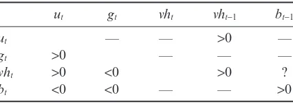
As the links among variables are often formed by combinations of
param-eters, it is useful to summarize the sign of links, as in the rows of table 4.
Most results are straightforward while some require a few additional
comments.
As wealth
vh
depends positively on
u
but negatively on
g
the overall impact
on wealth of an increase in the utilization rate that increases the growth rate
is ambiguous. The first derivative shows that
vh
will increase with
u
if
vh
> ⋅ − ⋅
µ
(
1
θ π α θ β
)
(
⋅ +
)
Therefore ‘small’ values of wealth imply a positive link between the
utiliza-tion rate and wealth itself, which is convenient for model stability: starting
Table 4. Short-run links among model variables
u
tg
tvh
tvh
t-1b
t-1u
t—
—
>
0
—
g
t>
0
—
—
—
vh
t>
0
<
0
>
0
?
from small values for
vh, a shock to the utilization rate cumulates through
higher wealth, which feeds back into higher utilization rates and faster
growth, but eventually, as wealth gets large enough, further increases in
u
will
reduce
vh
stabilizing the model.
The graph in figure 2 is drawn under the assumption that
vh
(and therefore
d) depend positively on
u.
The direct link between
vh
tand
vh
t-1is positive, unless households spend in
each period a fraction of their wealth
a
·
vh
t-1, which exceeds their stock of
deposits given by (1
-
d
) ·
vh
t-1, which is implausible. The overall impact of a
change in
vh
t-1on
vh
tis ambiguous, as shown in table 4, as it depends on the
relative size of the effects operating through
u
(see above);
vh
t-1(positive) and
g
(negative). From the discussion above, the size of the overall impact of the
opening stock of wealth on the closing stock of wealth will decrease with the
wealth level.
An increase in the opening stock of bills
b
t-1will decrease the stock of
wealth when the banks’ mark-up
t
bis ‘high’, i.e. when
τ
b>
µ
(
1
−
µ
)
Model stability requires that
d
b
t/
d
b
t-1<
1, which will be true when the growth
rate
g
is smaller than the interest rate
ib. Again, stability requires that
d
vh
t/
d
vh
t-1<
1 which cannot be ensured, but it is likely to hold when the
share of wealth spent on consumption is not too small relative to the size of
household deposits.
More formally, model stability can be analyzed with the help of phase
diagrams, reducing our system of four equations to a system in (the changes
of)
vh
and
b. Using (11) and (9) in (44) and (38) we get
Δ
vh
t=
f vh
1(
t−1;
b
t−1)
(48)
Δ
b
t=
f vh
2(
t−1;
b
t−1)
(49)
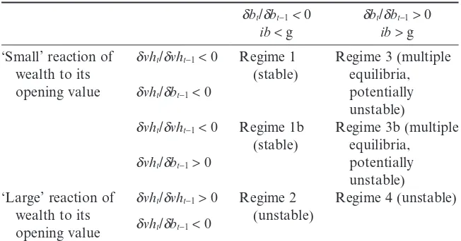
Inspection of the explicit functions in (48) and (49) reveals different
regimes, which may be either stable or unstable. Noting that
d
b
t/
d
vh
t-1<
0
always holds, we have six different regimes summarized in table 5.
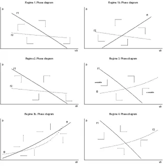
The phase diagrams for all regimes are shown in figure 3. We note that,
although Regimes 2 and 4 are theoretically possible, we have not been able
to generate them with any combination of parameters, because—as discussed
above—the relationship between
vh
tand
vh
t-1is likely to be small and
Summing up, the model admits at least one solution for economically
sensible values of parameters, and can produce multiple equilibria under
Regime 3. In most cases the model will thus converge to a long-run
equilib-rium, and in the next section we will investigate the properties of such
equilibrium.
3.3
The long-period equilibrium of the model and its interpretation
3.3.1
The long-period equilibrium
Define long-period equilibrium as the situation where our stock ratios
b,
l,
u
and
vh
are constant, for given interest rates. By virtue of (9), this will imply
steady growth. Applying these conditions to equations (9), (11), (38) and (44)
let us derive a system of two equations, either in
vh
and
u, or in
vh
and
b. Both
solutions are, of course, equivalent, but their graphical representation, and
their formal derivation, provide different insights that are worth exploring.
223.3.1.1
Deriving equations in
vh
and
u
The first long-run equilibrium condition can be obtained directly from (11),
solving for
vh. In the long run, there is a strictly positive relation between
22 See http://gennaro.zezza.it/papers/zds2007/ for details on deriving the two sets of equilibrium conditions.
Table 5. Possible model regimes
d
b
t/
d
b
t-1<
0
d
b
t/
d
b
t-1>
0
ib
<
g
ib
>
g
‘Small’ reaction of
wealth to its
opening value
d
vh
t/
d
vh
t-1<
0
Regime 1
(stable)
Regime 3 (multiple
equilibria,
potentially
unstable)
d
vh
t/
d
b
t-1<
0
d
vh
t/
d
vh
t-1<
0
Regime 1b
(stable)
Regime 3b (multiple
equilibria,
potentially
unstable)
d
vh
t/
d
b
t-1>
0
‘Large’ reaction of
wealth to its
opening value
d
vh
t/
d
vh
t-1>
0
Regime 2
(unstable)
Regime 4 (unstable)
wealth and the utilization rate, which does not depend on the composition of
wealth, but only on the effect of the interest rate on investment.
vh
=
[
u
ψ
1−
A ib
( )
]
a
(50)
The second equilibrium condition is obtained by substituting
u
into
b, and
both into
vh.
where
a
1is the accelerator from equation (13) and
α
2= ⋅ −
µ
(
1
θ π
)
⋅
(52)
ψ
2=
g
0− + +
[
1
(
1
τ
b)
⋅
θ
1]⋅
ib
(53)
ψ
3=
g
0−
[
θ
1+ −
(
1
δ
)
⋅ −
(
1
µ
)
]⋅ +
(
1
τ
b)
⋅ +
ib a
(54)
ψ
4= − +
1
(
1
τ
b)
⋅ −
(
1
µ
)
(55)
The system of equations (50) and (51) yields a cubic expression in
vh, which
confirms the possibility of multiple equilibria discussed above. Under Regime
1, our numerical analysis under a wide choice of parameters has shown that
only one solution implies economically meaningful values for all variables,
while under Regime 3 more than one (economically meaningful) solutions are
possible.
Our equation (50) has been derived directly from our equations for growth
equilibrium in the goods market, which is influenced by total wealth
vh, but
does not depend on the composition of wealth or by the levels of government
debt or by the stock of loans. We therefore label this curve
GME
for Goods
Markets Equilibrium in figure 4, as it gives the combination of utilization
rates
u
and wealth to capital ratio
vh
that imply steady growth for any
distribution of wealth.
As our second equation for long-run equilibrium has been derived, for
given (equilibrium) values of
u
and
g, through the equilibrium values for
b
and
vh, we will label this curve
FE
for Financial Equilibrium in figure 4.
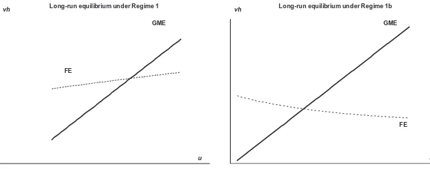
Equation (51) has a negative slope under Regime 1b, and a positive slope
under Regime 1. Under Regime 3 the slope of the
FE
curve varies with
u,
yielding multiple equilibria.
Long-run equilibrium under Regime 1
u vh
GME
FE
Long-run equilibrium under Regime 1b
u vh
GME
FE
3.3.1.2
Deriving equations in
vh
and
b
An alternative derivation of the long-run solution in the
b,
vh
space is also of
interest. Applying the steady-state conditions to equations (38) and (44) gives
us the following two new long-period equilibrium conditions:
ib b
⋅ + − ⋅
u b
g
(
γ θ
)
=
(56)
ib
⋅ +
(
b)
⋅ −
(
)
⋅ −
(
)
−
a vh
bib b
[
]⋅ + − +
[
(
)
⋅ −
(
)
]⋅ ⋅
+ ⋅ −
(
)
1
1
1
1
1
1
1
τ
δ
µ
τ
µ
µ
θ ⋅⋅ ⋅ =
π
u
g
(57)
The equations above simply state that steady growth is only possible when
the rate of growth of both government debt—implied by the government
deficit—and household wealth—implied by household saving—are equal to
the rate of growth of the capital stock
g.
23That is to say, the long-period equilibrium is such that
−
SAVg B
t t−1=
SAVh Vh
t t−1=
Δ
K K
t t−1Now note that replacing (9) in (56) and (57) gives us the following conditions,
which are an explicit form of the equations analyzed earlier for phase
diagrams:
b
=
(
ζ ζ
1− ⋅
2vh
)
(
ζ
3+ ⋅
ζ
4vh
)
(58)
b
=
(
ζ ζ
4 7)
⋅
vh
+
(
ζ ζ
)
⋅ +
vh
(
ζ ζ
)
2
5 7 6 7
(59)
where:
ζ
1= − ⋅ ⋅
γ θ
A
ψ
1(60)
ζ
2= ⋅ ⋅
θ
a
ψ
1(61)
ζ
3= ⋅ + ⋅
A
(
1
α ψ
1 1)
− −
γ
ib
(62)
ζ
4=
α
1⋅ ⋅
a
ψ
1(63)
ζ
5=
ψ ψ
0⋅ ⋅ − ⋅ +
1A ib
(
1
τ
b)
⋅ −
(
1
δ
)
⋅ −
(
1
µ
)
+ ⋅ −
a
[
1
ψ
1⋅ −
(
1
θ µ π
)
⋅ ⋅
] −
γ
(64)
ζ
6= −
(
1
θ µ π ψ
)
⋅ ⋅ ⋅ ⋅
1A
(65)
23 Note that the fact thatpe