Electronic Journal of Qualitative Theory of Differential Equations
2009, No. 52, 1-13;http://www.math.u-szeged.hu/ejqtde/
APPROXIMATION OF SOLUTIONS OF NONLINEAR HEAT TRANSFER PROBLEMS
RAHMAT ALI KHAN
Centre for Advanced Mathematics and Physics, National University of Sciences and Technology(NUST), Campus of College of Electrical and Mechanical Engineering,
Peshawar Road, Rawalpindi, Pakistan, rahmat
Abstract. We develop a generalized approximation method (GAM) to obtain solution of a steady state one-dimensional nonlinear convective-radiative-conduction equation. The GAM generates a bounded monotone sequence of solutions of linear problems. The sequence of approximants converges monotonically and rapidly to a solution of the original problem. We present some numerical simulation to illustrate and confirm our results.
Keywords: heat transfer equations, upper and lower solutions, generalized approximation method
1. Introduction
Most metallic materials have variable thermal properties, usually depending on tempera-ture. The governing equations describing the temperature distribution along such surfaces are nonlinear. In consequence, exact analytic solutions of such nonlinear problems are not available in general. Scientists use some approximation techniques for example, perturbation method [7], [25], homotopy perturbation method [1], [3], [5], [12], [13], [14] , [24], to approx-imate solutions of the nonlinear problems. However, these methods have the drawback that the series solutions may not always converge to a solution of the problem and, in some cases, produce inaccurate and meaningless results.
In this paper, we develop the generalized approximation method (GAM), [2], [6], [15], [16], [17], to approximate solutions of nonlinear problems. This method produces excellent result and is independent of the choice of a small parameter. It generates a bounded monotone sequence of solutions of linear problems which converges uniformly and rapidly to a solution
Acknowledgement: The author is thankful to the referee for valuable comments and suggestions that improve the manuscript.
Research is supported by HEC, Pakistan.
of the original problem. Hence it can be applied to a much larger class of nonlinear boundary value problems. Moreover, we show that our results are consistent and accurately represent the actual solution of the problem for any value of the parameter. For the numerical simula-tion, we use the computer programme, Mathematica. For computational purposes, the linear iteration is important. The generalized approximation method which uses linear problems is a particular version of the well studied quasilinearization method [8, 9, 10, 18, 19, 20, 21]. At each iteration, we are dealing with linear problems and obtain a monotone sequence of solutions of linear problems which converges to a solution of the original nonlinear problem.
2. HEAT TRANSFER PROBLEM: INTEGRAL FORMULATION
Consider a straight fin of lengthLmade of materials with temperature dependent thermal conductivity k = k(T). The fin is attached to a base surface of temperature Tb extended into a fluid of temperatureTa withTb > Ta and its tip is insolated. Assume that the thermal conductivity k vary linearly with temperature, that is,
(2.1) k(T) =ka[1 +η(T −Ta)],
where η is constant and ka is the thermal conductivity at temperature Ta. Choose the tip of the fin as originx= 0 and the base of the fin at position x=L. The fin surface transfers heat through convection, conduction and radiation. Assume that the emissivity coefficient of the surface Eg is constant and the convective heat transfer coefficient h depends on the temperature. The convective heat transfer coefficient h usually varies as a power law of the type,
(2.2) h=h(T) =hb(
T −Ta
Tb−Ta )n,
see [23], where hb is the heat transfer coefficient at the base temperature and the number n depends on the heat transfer mode. For example, for laminar film boiling or condensation
n=−1/4, for laminar natural convectionn= 1/4, for turbulent natural convection n= 1/3, for nucleate boiling n = 2 and for radiation n = 3. Here, we restrict our study to the case
n > 1 and T ≥ Ta. Our results are also valid for the case n ≤1 but with possibly different upper and lower solutions.
The energy equation describing one dimensional steady state temperature distribution is given by
d dx
k(T)dT
dx
− ph
A(T −Ta)− Egσ
A (T −Ta)
4 = 0, x∈[0, L],
dT
dx(0) = 0, T(L) =Tb,
(2.3)
see [11] and [22], where Ais the cross-sectional area and pis a parameter of the fin. In view of (2.1) and (2.2), the boundary value problem (2.3) can be rewritten as follows
d dx
(1 +η(T −Ta))dT
dx
− phb Aka
(T −Ta)n+1
(Tb−Ta)n
−Egσ Aka
(T −Ta)4 = 0, x∈[0, L],
dT
dx(0) = 0, T(L) =Tb,
Introducing the dimensionless quantities θ = T−Ta Tb−Ta, y =
x
L, we obtain
d dy
(1 +ǫ1θ) dθ dy
−Nθn+1−ǫ
2θ4 = 0, y ∈[0,1],
dθ
dy(0) = 0, θ(1) = 1,
(2.4)
where, ǫ1 =η(Tb−Ta), N = hbpL
2
kaA and ǫ2 =
L2E
gσ(Tb−Ta)3
kaA . From the definition ofθ, we have
θ ≥ 0. From the differential equation in (2.4), we obtain dyd[(1 +ǫ1θ)dθdy]≥ 0, which implies
that the function (1 +ǫ1θ)dθdy in nondecreasing on [0,1]. Hence using the boundary condition
at 0, it follows that dθ
dy ≥ 0, that is, the function θ is monotonically increasing on [0,1]. Hence, 0 ≤ θ(y) ≤ θ(1) = 1, y ∈ [0,1] and these provide bounds for the possible solutions of the BVP (2.4). Moreover, from (2.4), we obtain d2θ
dy2 ≥ −
ǫ1(dydθ)2
1+ǫ1θ , which implies that the
function dθdy may not be monotone on [0,1].
Now, for simplicity, we write the problem (2.4) as follows
−d 2θ dy2 =
ǫ1(dθdy)
2−Nθn+1−ǫ 2θ4
(1 +ǫ1θ)
, y ∈[0,1] =I,
θ′(0) = 0, θ(1) = 1,
(2.5)
which can be written as an equivalent integral equation
θ(y) = 1 +
Z 1
0
G(y, s)ǫ1(
dθ dy)
2−Nθn+1−ǫ 2θ4
(1 +ǫ1θ)
]ds = 1 +
Z 1
0
G(y, s)f(θ, θ′),
(2.6)
where f(θ, θ′) = ǫ1( dθ dy)
2
−N θn+1
−ǫ2θ4 (1+ǫ1θ) and
G(y, s) =
1−s, 0≤y < s ≤1,
1−y, 0≤s < y ≤1,
is the Green’s function. Clearly,G(y, s)>0 on (0,1)×(0,1).
Recall the concept of lower and upper solutions corresponding to the BVP (2.5).
Definition 2.1. A function α ∈ C1(I) is called a lower solution of the BVP (2.5), if it
satisfies the following inequalities,
−α′′(y) ≤f(α(y), α′(y)), y∈(0,1)
α′(0)≥0, α(1)≤1.
An upper solution β ∈C1(I) of the BVP (2.5) is defined similarly by reversing the
inequal-ities.
For example, α= 0 andβ = 1 are lower and upper solutions of the BVP (2.5) respectively as they satisfy the inequalities:
α′′(y) +f(α, α′) = 0, y ∈I, α′(0) = 0, α(1)<1
β′′(y) +f(β, β′) = −(N +ǫ2)
1 +ǫ1
<0, y ∈I, β′(0) = 0, β(1) = 1.
For broad variety of nonlinear boundary value problems, it is possible to find a solution between the lower and the upper solutions. To give an estimate of the derivative u′ of a
possible solution, we recall the concept of Nagumo function.
Definition 2.2. A continuous function ω: (0,∞)→(0,∞) is called a Nagumo function if
Z ∞
λ
sds
ω(s) =∞,
for λ = max{|α(0)−β(1)|,|α(1)−β(0)|}. We say that f ∈ C[R×R] satisfies a Nagumo condition relative to α, β if for y ∈ [minα,maxβ], there exists a Nagumo function ω such that |f(y, y′)| ≤ω(|y′|).
Forθ ∈[0,1] = [minα,maxβ], we have
|f(θ, θ′)| ≤ǫ
1|θ′|2+N +ǫ2 =ω(|θ′|)
and
Z ∞
1 sds ω(s) =
Z ∞
1
sds ǫ1s2+N +ǫ2
=∞,
which implies that f satisfies a Nagumo condition with ω(s) =ǫ1s2+N +ǫ2 as a Nagumo
function. Hence by Theorem 1.4.1 of [4] (page 14) , there exists a constantC > λsuch that any solutionθ of the BVP (2.4) which satisfies α≤θ ≤β on I, must satisfies |θ′| ≤C onI.
Using the relation RC 1
sds
ω(s) ≥ maxβ−minα = 1, we obtain C ≥ [e
2ǫ1 + (e2ǫ1 −1)N+ǫ2
ǫ1 ] 1 2.
In particular, we may chooseC = [e2ǫ1+ (e2ǫ1−1)N+ǫ2
ǫ1 ] 1
2. Hence, any solution θ of the BVP
(2.4) such that 0≤θ ≤1 satisfies |θ′| ≤C and this provide estimate for the derivative of a
solutionθ.
The following result is known [4] (Theorem 1.5.1, Page 31).
Theorem 2.3. Assume that α, β ∈ C1(I) are lower and upper solutions of the BVP (2.4) such that α ≤ β on I. Assume that f : R ×R → (0,∞) is continuous and satisfies a Nagumo’s condition on I relative to α, β. Then the BVP (2.4) has a solution θ ∈ C1(I) such that α≤θ ≤β and |θ′| ≤C on I, where C depends only on α, β and h.
We note that the BVP (2.4) satisfies the conditions of Theorem 2.3 with α= 0 and β = 1 as lower and upper solutions.
3. GENERALIZED APPROXIMATION METHOD (GAM)
Notice that fθ(θ, θ′) =−(N(n+1)nθn+4ǫ2θ3+N nǫ1θn+1+3ǫ1ǫ2θ4+ǫ1θ′2)
(1+ǫ1θ)2 <0,fθ′(θ, θ
′) = 2ǫ1θ′ (1+ǫ1θ),
fθθ(θ, θ′) =
2ǫ1(N2+ǫ21θ′2)−2(6 + 8ǫ1θ+ 3ǫ21θ2)ǫ2θ2
(1 +ǫ1θ)3
,
fθ′θ′(θ, θ′) = 2ǫ1
1 +ǫ1θ
and fθθ′(θ, θ′) =
−2ǫ2 1θ′
(1 +ǫ1θ)2 .
(3.1)
Hence, the quadratic form
vTH(f)v = (θ−z)2fθθ(z, z′) + 2(θ−z)(θ′−z′)f
θθ′(z, z′) + (θ′−z′)2fθ′θ′(z, z′)
=(θ−z)
s
2ǫ3z′2
(1 +ǫz)3 −(θ
′−z′)
s
2ǫ1
(1 +ǫ1z) 2
+ (θ−z)
2
(1 +ǫ1z)3
[Nǫ1(nǫ1(n−ǫ1) + 2)zn]
− (θ−z) 2
(1 +ǫ1z)3 R(z),
(3.2)
whereR(z) = [2ǫ2z2(6+8ǫ1z+3ǫ21z2)+(n(n+1)+2n2z)Nzn−1],H(f) =
fθθ fθθ′
fθθ′ fθ′θ′
!
is the
Hessian matrix andv = θ−z
θ′−z′
!
. If the quadratic formvTH(f)v 0 on [minα,maxβ]×
[−C, C], then we need to choose an auxiliary function φ such that vTH(F)v ≥ 0 on [minα,maxβ]×[−C, C], where F = f +φ. In our case, we choose φ(θ) = m2(z)θ2, where m(z) = 2ǫ2z2(6 + 8ǫ1z+ 3ǫ21z2) +n(3n+ 1)N ≥R(z). Hence,
(3.3) vTH(F)v ≥0, on [minα,maxβ]×[−C, C],
which implies that
F(θ, θ′)≥F(z, z′) +Fθ(z, z′)(θ−z) +F
θ′(z, z′)(θ′−z′), (3.4)
where z, θ∈[minα, maxβ] = [0,1], z′, θ′ ∈[−C, C], which further implies that
f(θ, θ′)≥f(z, z′) +Fθ(z, z′)(θ−z) +F
θ′(z, z′)(θ′−z′)−(φ(θ)−φ(z)). (3.5)
Using the relation φ(θ)−φ(z) = m(2z)(θ+z)(θ−z)≤m(z)(θ−z) forθ ≥z, we obtain
f(θ, θ′)≥f(z, z′) + (Fθ(z, z′)−m(z))(θ−z) +f
θ′(z, z′)(θ′−z′), forθ ≥z.
Now,
Fθ(z, z′)−m(z) =−h(N(n+ 1)nz
n+ 4ǫ
2z3+Nnǫ1zn+1+ 3ǫ1ǫ2z4 +ǫ1z′2)
(1 +ǫ1z)2
+ (1−z)m(z)i
≥ −m1,
where,
m1 = max{
(N(n+ 1)nzn+ 4ǫ
2z3+Nnǫ1zn+1+ 3ǫ1ǫ2z4 +ǫ1z′2)
(1 +ǫ1z)2
+ (1−z)m(z) :
z ∈[0,1], z′ ∈[−C, C]}.
Hence,
f(θ, θ′)≥f(z, z′)−m
1(θ−z) +fθ′(z, z′)(θ′ −z′), for θ ≥z. (3.6)
Define g :R4 →R by
g(θ, θ′; z, z′) =f(z, z′)−m
1(θ−z) +fθ′(z, z′)(θ′−z′) =q(z)−m1θ+p(z)θ′, (3.7)
where p(z) = 2ǫ1z′
1+ǫ1z, q(z) =m1z−
ǫ1z′2+N zn+1+ǫ2z4 1+ǫz .
Clearly, g is continuous and satisfies the following relations
(3.8)
f(θ, θ′)≥g(θ, θ′; z, z′) for θ≥z,
f(θ, θ′) =g(θ, θ′; θ, θ′),
where θ, z ∈ [0,1], θ′, z′ ∈ ×[−C, C]. We note that for every θ, z ∈ [0, 1] and z′ ∈ some
compact subset of R, g satisfies a Nagumo condition relative to α, β. Hence, there exists a constant C1 such that any solution θ of the linear BVP
−θ′′(y) = g(θ, θ′; z, z′) =q(z)−m
1θ+p(z)θ′, y ∈I, θ′(0) = 0, θ(1) = 1,
(3.9)
with the property that α ≤ θ ≤ β on I, must satisfies |θ′| < C
1 on I. We note that the
linear problem (3.9) can be solved analytically.
To develop the iterative scheme, we choose w0(y) = α(y) = 0 as an initial approximation
and consider the following linear BVP
−θ′′(y) = g(θ, θ′; w
0, w′0) =−m1θ, y∈I, θ′(0) = 0, θ(1) = 0,
(3.10)
whose solution is w1(y) = cosh(
√m
1y) cosh(√m1).
In general, using (3.8) and the definition of lower and upper solutions, we obtain
g(w0, w0′; w0, w0′) = f(w0, w0′)≥ −w0′′,
g(β, β′; w
0, w0′)≤f(β, β′)≤ −β′′, on I,
which imply thatw0 and β are lower and upper solutions of (3.10). Hence, by Theorem 2.3,
there exists a solution w1 of (3.10) such that w0 ≤w1 ≤β, |w1′|< C1 on I. Using (3.8) and
the fact that w1 is a solution of (3.10), we obtain
(3.11) −w′′
1(y) =g(w1, w1′; w0, w0′)≤f(w1, w1′)
which implies thatw1 is a lower solution of (2.4). Similarly, we can show thatw1 and β are
lower and upper solutions of
−θ′′(y) = g(θ, θ′; w
1, w1′), y ∈I, θ′(0) = 0, θ(1) = 1.
(3.12)
Hence, there exists a solutionw2 of (3.12) such that w1 ≤w2 ≤β, |w2′|< C1 on I.
Continuing this process we obtain a monotone sequence {wn} of solutions satisfying
α=w0≤ w1 ≤w2 ≤w3 ≤...≤wn−1 ≤wn ≤β, |wn′| < C1 onI,
where wn is a solution of the linear problem
−θ′′(y) =g(θ, θ′; w
n−1, wn′−1), y ∈I
θ′(0) = 0, θ(1) = 1
and is given by
(3.13) wn(y) = 1 +
Z 1
0
G(y, s)g(wn(s), w′
n(s);wn−1(s), wn′−1(s))ds, y ∈I.
The sequence of functionswnis is uniformly bounded and equicontinuous. The monotonicity and uniform boundedness of the sequence {wn} implies the existence of a pointwise limit w onI. From the boundary conditions, we have
0 =w′
n(0)→w′(0) and 1 =wn(1)→w(1).
Hencewsatisfy the boundary conditions. Moreover, by the dominated convergence theorem, for any y∈I,
Z 1
0
G(y, s)g(wn(s), w′
n(s); wn−1(s), wn′−1(s))ds→ Z 1
0
G(y, s)f(w(s), w′(s))ds.
Passing to the limit as n→ ∞, we obtain
w(y) = 1 +
Z 1
0
G(y, s)f(w(s), w′(s))ds, y∈I,
that is, wis a solution of (2.4).
Hence, the sequence of approximants {wn} converges to the unique solution of the non-linear BVP (2.4). Moreover, the convergence is quadratic, see [16], [17]. The fact that the sequence converges rapidly to the solution of the problem can also be seen from the numerical experiment.
4. NUMERICAL RESULTS FOR GAM, HPM and VIM
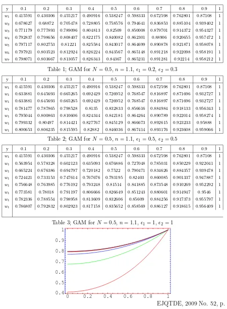
Starting with the initial approximationw0 = 0 and setN = 0.5, n= 1.1, results obtained
via GAM for (ǫ1 = 0.2ǫ2 = 0.3), ǫ1 = 0.5ǫ2 = 0.5 and ǫ1 = 1ǫ2 = 1 are shown in Tables
(Table 1, Table 2 Table 3 respectively) and also graphically in Fig.1, Fig.2 and Fig.3. Form the tables and graphs, it is clear that with only few iterations it is possible to obtain good approximations of the exact solution. Moreover, the convergence is very fast. Even for larger values of N, n, the GAM produces excellent results and fast convergence, see for example, Fig.5, Fig 6 and Fig.7. In fact, the GAM accurately approximate the actual solution of the problem independent of the choice of the parameters ǫ1 and ǫ2 involved, Fig. 4 and Fig. 8.
y 0.1 0.2 0.3 0.4 0.5 0.6 0.7 0.8 0.9 1
w1 0.415591 0.430306 0.455217 0.490916 0.538247 0.598333 0.672598 0.762801 0.87108 1
w2 0.678627 0.68872 0.705478 0.728805 0.758576 0.794641 0.836853 0.885104 0.939402 1
w3 0.771179 0.777893 0.789096 0.804813 0.82509 0.850008 0.879701 0.914372 0.954327 1 w4 0.792837 0.798656 0.808407 0.822175 0.840082 0.862301 0.88906 0.920655 0.957472 1
w5 0.797117 0.802753 0.81221 0.825584 0.843017 0.864699 0.890878 0.921871 0.958078 1
[image:9.595.83.533.114.727.2]w6 0.797921 0.803523 0.812924 0.826224 0.843567 0.865148 0.891218 0.922098 0.958191 1 w7 0.798071 0.803667 0.813057 0.826343 0.84367 0.865231 0.891281 0.92214 0.958212 1
Table 1; GAM forN = 0.5, n= 1.1, ǫ1 = 0.2, ǫ2= 0.3
y 0.1 0.2 0.3 0.4 0.5 0.6 0.7 0.8 0.9 1
w1 0.415591 0.430306 0.455217 0.490916 0.538247 0.598333 0.672598 0.762801 0.87108 1 w1 0.633881 0.645693 0.665265 0.692429 0.726952 0.768547 0.816897 0.871696 0.932727 1
w1 0.633881 0.645693 0.665265 0.692429 0.726952 0.768547 0.816897 0.871696 0.932727 1
w1 0.781477 0.787865 0.798528 0.8135 0.832833 0.856616 0.884984 0.918133 0.956343 1
w1 0.795044 0.800863 0.810606 0.824344 0.842181 0.864264 0.890789 0.922014 0.958274 1
w1 0.799332 0.80497 0.814421 0.827767 0.845129 0.866673 0.892615 0.923233 0.95888 1 w1 0.800653 0.806235 0.815595 0.82882 0.846036 0.867414 0.893176 0.923608 0.959066 1
Table 2; GAM forN = 0.5, n= 1.1, ǫ1 = 0.5, ǫ2= 0.5
y 0.1 0.2 0.3 0.4 0.5 0.6 0.7 0.8 0.9 1
w1 0.415591 0.430306 0.455217 0.490916 0.538247 0.598333 0.672598 0.762801 0.87108 1
w1 0.563954 0.578328 0.602123 0.635093 0.676886 0.727048 0.785031 0.850229 0.922041 1
w1 0.665224 0.676386 0.694797 0.720182 0.7522 0.790471 0.834626 0.884357 0.939478 1 w1 0.724421 0.733153 0.747614 0.767676 0.793195 0.82403 0.860085 0.901337 0.947887 1
w1 0.756648 0.763985 0.776192 0.793248 0.81514 0.841885 0.873548 0.910269 0.952292 1
w1 0.773581 0.78018 0.791197 0.806666 0.826649 0.851243 0.880601 0.914947 0.9546 1 w1 0.782336 0.788554 0.798958 0.813609 0.832606 0.85609 0.884256 0.917373 0.955797 1
w1 0.786807 0.792832 0.802923 0.817158 0.835652 0.858569 0.886127 0.918615 0.956409 1
Table 3; GAM for N = 0.5, n= 1.1, ǫ1 = 1, ǫ2= 1
0 0.2 0.4 0.6 0.8 1
0.4 0.5 0.6 0.7 0.8 0.9 1
Fig.1, [N = 0.5, n = 1.1,], results via GAM for ǫ1 = 0.2, ǫ2 = 0.3
0 0.2 0.4 0.6 0.8 1
0.4 0.5 0.6 0.7 0.8 0.9 1
Fig.2, [N = 0.5, n= 1.1], results via GAM for ǫ1 = 0.5, ǫ2 = 0.5
0 0.2 0.4 0.6 0.8 1
0.4 0.5 0.6 0.7 0.8 0.9 1
Fig.3, [N = 0.5, n= 1.1], results via GAM for ǫ1 = 1, ǫ2 = 1
0 0.2 0.4 0.6 0.8 1
0.8 0.85 0.9 0.95 1
Fig.4,N = 0.5, n = 1.1],GAM for ǫ1 = 0.2, ǫ2 = 0.3 (Red),ǫ1 = 0.5, ǫ2 = 0.5 (Green) and ǫ1 = 1, ǫ2 = 1 (Blue)
0 0.2 0.4 0.6 0.8 1 0
0.2 0.4 0.6 0.8 1
Fig.5, [N = 1, n= 2], results via GAM for ǫ1 = 0.2, ǫ2 = 0.3
0 0.2 0.4 0.6 0.8 1
0 0.2 0.4 0.6 0.8 1
Fig.6, [N = 1, n= 2], results via GAM for ǫ1 = 0.5, ǫ2 = 0.5
0 0.2 0.4 0.6 0.8 1
0 0.2 0.4 0.6 0.8 1
Fig.7, [N = 1, n= 2], results via GAM for ǫ1 = 1, ǫ2 = 1
0 0.2 0.4 0.6 0.8 1 0.75
0.8 0.85 0.9 0.95 1
Fig.8,N = 1, n = 2],GAM for ǫ1 = 0.2, ǫ2 = 0.3 (Red), ǫ1 = 0.5, ǫ2 = 0.5 (Green) and ǫ1 = 1, ǫ2 = 1 (Blue)
5. Conclusion
In this paper, the GAM is developed for the heat flow problems. The GAM generates a bounded monotone sequence of solutions of linear problems that converges monotonically and rapidly to a solution of the original problem. It also ensure existence of solution with lower and upper solutions as estimates for the exact solution. It does not require the existence of small or large parameter as most of the perturbation type methods do. The results obtained via GAM are accurate for any value of the parameters involved. Hence it is a powerful tool for solutions of nonlinear problems.
References
[1] O. Abdulaziz, I. Hashim and S. Momani, Application of homotopy-perturbation method to fractional IVPs Journal ofComputational and Applied Mathematics, 216(2008), 574-584.
[2] B. Ahmad and J. J. Nieto, Existence and approximation of solutions for a class of nonlinear impulsive functional differential equations with anti-periodic boundary conditions, Nonlinear Analysis: Theory, Methods and Applications, doi:10.1016/j.na.2007.09.018
[3] A. Belendez, C. Pascual, A. Marquez and D.I. Mendez, Application of He’s Homotopy Perturbation Method to the Relativistic (An)harmonic Oscillator. I: Comparison between Approximate and Exact Frequencies,International Journal of Nonlinear Sciences and Numerical Simulation 8(2007), 483-492.
[4] Stephen R. Bernfeld and V. Lakshmikantham, An introduction to nonlinear boundar value problems, Academic Press, Inc. New Yark and Landa (1974).
[5] A. Belendez, C. Pascual, D.I. Mendez, M.L. Alvarez and C. Neipp , Application of He’s Homotopy Perturbation Method to the Relativistic (An)harmonic Oscillator. II: A More Accurate Approximate Solution,International Journal of Nonlinear Sciences and Numerical Simulation 8(2007), 493-504.
[6] A. Cabada and J. J. Nieto, Quasilinearization and rate of convergence for higher-order nonlinear periodic boundary-value problems,Journal of Optimization Theory and Applications 108 (2001), 97-107
[7] M. Van Dyke, Perturbation Methods in Fluid Mechanics, Annotated Edition, Parabolic Press, Stand-ford, CA, (1975).
[8] P. W. Eloe and Yang Gao, The method of quasilinearization and a three-point boundary value problem, J. Korean Math. Soc.,39(2002), 319–330.
[9] P. W. Eloe, The quasilinearization method on an unbounded domain, Proc. Amer. Math. Soc.,
131(2002)5 1481-1488.
[10] P. W. Eloe and Y. Zhang, A quadratic monotone iteration scheme for two point boundary value problems for ordinary differential equations,Nonlinear Anal.,33(1998) 443-453.
[11] D. D. Ganji and A. Rajabi, Assessment of homotopy perturbation method in heat radiation equations, Int. Commun. heat and Mass transfer 33(2006),391–400. doi:10.1016/j.cnsns.2007.09.007.
[12] J. H. He, Homotopy perturbation technique,Comput.Methods Appl. Mech. Eng.,178(1999)(257), 3–4.
[13] J. H. He, A coupling method of a homotopy technique and a perturbation technique for non-linear problems,Int. J. Nonlinear Mech., 35(2000),37–43 .
[14] B. Keramati, An approach to the solution of linear system of equations by He’s homotopy perturbation method,Chaos, Solitons and Fractals, In Press, doi:10.1016/j.chaos.2007.11.020.
[15] R. A. Khan, Generalized quasilinearization for periodic problems, Dyn. Contin. Discrete Impuls. Syst. Ser. A Math. Anal.14(2007), 497-507.
[16] R. A. Khan, Generalized approximations method for heat radiation equations, Appl. Math. Comput., Doi:10.1016/j.amc.2009.02.028.
[17] R. A. Khan, The Generalized approximations and nonlinear heat transfer equations,Elec. J. Qualitative theory of Diff. Equations,2(2009), 1–15.
[18] V. Lakshmikantham and A.S. Vatsala, Generalized quasilinearization for nonlinear problems, Kluwer Academic Publishers, Boston (1998).
[19] V. Lakshmikanthama and A.S. Vatsala, Generalized quasilinearization versus Newtons method, Appl. Math. Comput.164(2005), 523-530.
[20] V. Lakshmikantham, An extension of the method of quasilinearization, J. Optim. Theory Appl., 82
(1994), 315–321.
[21] V. Lakshmikantham, Further improvement of generalized quasilinearization,Nonlinear Anal.,27(1996),
315–321.
[22] Mo. Miansari, D. D. Ganji and Me.Miansari, Application of He’s variational iteration method to non-linear heat transfer equations,Physics Letter A,372(2008), 779-785.
[23] S. Kim and C-H. Huang, A series solution of the non-linear fin problem with temperature-dependent thermal conductivity and heat transfer coefficient,J. Phys. D: Appl. Phys., 40(2007) 2979-2987.
[24] Xiaoyan Ma, Liping Wei and Zhongjin Guo, He’s homotopy perturbation method to periodic solutions of nonlinear Jerk equations,Journal of Sound and Vibration 314(2008), 217-227.
[25] A. H. Nayfeh, Perturbation Methods, Wiley, New York, (1973).
(Received April 21, 2009)