www.elsevier.com/locate/physa
Penna model in migrating population – eect of
environmental factor and genetics
Maria S. Magdon
a;∗, Andrzej Z. Maksymowicz
baDepartment of Mathematical Statistics, Agriculture University, al. Mickiewicza 21,
31-120 Cracow, Poland
bDepartment of Physics and Nuclear Techniques, AGH, al. Mickiewicza 30, 30-059 Cracow, Poland
Received 31 May 1999
Abstract
We consider eect of possible migration between dierent locations on population evolution. Examples of dierent rules based on preferences to live in bigger or smaller populations, (or environmental capacity, or living space available), are discussed. In the limiting case of small migration intensity, each location evolves independently according to its local rules and con-ditions, as expected. With increasing migration, the population distribution between locations changes, including some critical behavior of extinction of population in some locations for spe-cic set of the rules. Then the deserted location may become populated again if the migration is still on increase as a result of a pressure to move. Presented version is devoted to the migration controlled exclusively by environmental factor, yet the model is primarily designed to describe inuence of other factors which may control migrating processes such as inherited mutation load, age, or other parameters associated either with individuals or the specic location, races mixing, or recovery of environmental capacity. c 1999 Elsevier Science B.V. All rights reserved.
PACS: 89.60.+x; 05.45.-a
Keywords:Penna model; Population evolution; Logistic equation; Migration
1. Introduction
In the simplest logistic model, population evolution may be described in terms of the normalized to the environmental capacity N populationn(t)¡ N at time (t). Then
x(t+ 1) = (1 +B)x(1−x); (1)
∗Corresponding author. Tel.: +48-632-16-20 extn. 261. E-mail address: [email protected] (M.S. Magdon)
where the right-hand side x=n=N is at timet. This equation predicts single value equi-libriumx=B=(1 +B) at growth rates 0¡ B ¡2, followed by cyclic solutions for larger B and then a chaotic regime. However, it must be noted that in computer simulation we apply probabilistic rules for the system evolution, and so the deterministic version of the logistic equation must be replaced by its version with some noise admixture ; x(t+ 1) = (1 +B)x(1−x) +. This mimics draws for the elimination (known as the
Verhulst factor [1]) of an individual due to the limited environmental capacity instead of purely deterministic recipe. As a result, we may not recover in the simulation cyclic behavior which may be suppressed by the noise.
The Penna model [2,3], may be considered as a generalization of the logistic picture for the case when the evolution rules include actual age a of an individual. Then populationx(t; a) may be considered as dierent groups of dierent ages, and after one time step we get x(t+ 1; a+ 1). In the Penna model each individual is characterized by an inherited genome which already possesses and anticipates all the future life of the individual. The genome is a computer word which contains information of ‘bad’ mutations prescribed for the individual’s whole future life. At the beginning, the mutations are idle and become activated by ow of time, one piece of information read from genome per each time step, and adding up to the already active number of mutations. On entry to the next era we scan over all members and eliminate the ones which are too old, or have too manyactivemutations (above thresholdT) or are hunted out, or perhaps for limited environmental capacity (the Verhulst factor). However, if the individual survives, it may give birth with probability B if the reproduction age R is reached. The baby’s genome is inherited from the parent, and gets M additional mutations randomly picked over its whole lifespan.
Thus dynamics of population n(t; a) is governed by a genetic load, environmental capacity N, the growth rate B and the minimum reproduction age R, bad mutation threshold T, the extra mutations M for the newly born and other parameters which make the rules on how the system evolves. A strong advantage of the Penna model is its exibility which makes it easy to produce specic versions devoted to some picked out scenario. This allows to study the role of dierent factors such as inuence of sexual selection, parental care, overshing or hunting etc., on the population [4,5].
In this paper we intend to account for migration in the population split into several locations and with possible transfer of individuals between these locations.
2. Model
We consider a number of locations labeled by i, each with its own set of evolution parameters. One iteration step leading from normalized populationxi(t) =ni=Ni at time
t to xi(t+ 1) is then a result of a scan over the whole population. For each item in
the population we consider
• : : : start from xi(t): : :
• giving birth
• : : : nish at xi(t+ 1).
This is the Penna model which we apply for siteration steps. This yields a new pop-ulation yi=xi(t+s). Then after a given number s of evolution steps, we also allow
each individual to migrate from location ito another locationjwith probability p(i; j). The probability p(i; j) is negotiable according to variety of scenarios which may be claimed or justied. After all migration moves are carried out, the full iteration cycle is complete:
• : : : from xi(t), by elimination followed by growth, s-times, to yi=xi(t+s): : : • : : : from yi=xi(t+s), by migration, to xi(t+s):
Obviously, forp(i; j) = 0 the game describes independent sub-populations and the stan-dard Penna model applies to each location. However, when migration is allowed, a new equilibrium is established which may be dierent from the isolated islands case. In the limiting case of logistic equation R= 0; M = 0 and large threshold T, the population yi after elimination and growth is expected to be
yi=kixi(1−xi); (2)
and the antisymmetrical transfer matrix Tij=−Tji is
Tij=
Nj
Nyjp(j; i)− Ni
Nyip(i; j): (5)
The rst term represents the inow of population into ith location from any location j, while the other term is the opposite. As we said, p(i; j) stands for the probability of an individual to migrate from location i to location j. In the following we conned ourselves to the uncorrelated version when at time (t+s) just before migration, the transfer matrix vanishes and so we get the claimed random migration for which xi(t+s) =yi, according to the Penna scheme
random migration
q(i) =q; p(j)˙yjNj=N ; (8)
where yjNj is the population at time (t+s) after executing the s evolution steps with
no migration, and just before the nal step of virtual migration which closes the full cycle of evolution,
• : : : x(t)→(s-steps of elimination and growth)→y→(migration)→x(t+s):
The neutral or random migration means x(t+s) =y. For non-random migration we choose probabilities of the migration dierent from the ones leading to the random moves. For example, for
q(i) =q=(yiNi=N); (9)
where q is a proportionality constant, then the total number of the ‘move-out-of’ indi-viduals is the same for each location, and independent of the actual population there. This is a resemblance of a ‘quota’ limit policy for migrating people, and the same for all locations, which may lead to faster escape of individuals from already deserted areas. As a result we expect a new equilibrium between locations with a tendency to clustering. Perhaps it is illustrative to consider the stability of the coupled (by migration process) two identical locations in the simple logistic case. Obviously yi=yj is the
solution. However, if a small uctuation (t) is allowed, so that one of the locations has a surplus of population, xi+, at the cost of the other location population, xj−,
then the system response after one full cycle with (t+s) =r(t). The ratio r may be obtained for the pure logistic equation as
r= (1−B) + (1−B)(q=qmax); qmax= 2B=(1 +B); (10)
with maximumqcoecient so that the probability is less that one. The system becomes unstable for the mobility parameterqlarger then a minimumqmin value whenrexceeds
one. This yields the instability regime for q,
0¡ B2=(1−B2)¡2q ¡ B=(1 +B); 0¡ B ¡0:5: (11)
Let us summarize the main concept. In the above example we claimed modication of the migration probability, as compared against the reference random transfers, according to some environmental factors such as the actual population yiNi.
This may serve as indication of what may be expected from computer simulation, also for the non-logistic version based on the Penna model. Actually, the dierences from the simulations show that positions of critical qc for the phase transitions are
similar for the Penna and the logistic case.
3. Results and conclusions
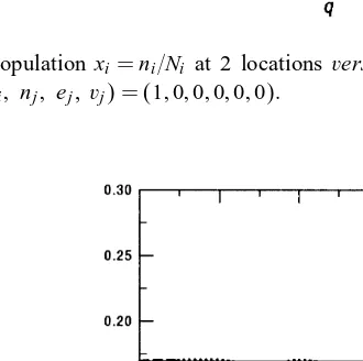
Fig. 1. Normalized population xi=ni=Ni at 2 locationsversusmobilityq, logistic case for set of the model parameters (ni; ei; vi; nj; ej,vj) = (1;0;0;0;0;0).
Fig. 2. Normalized population xi=ni=Ni at 2 locationsversus mobilityq, Penna case for set of the model parameters (ni; ei; vi; nj; ej; vj) = (1;0;0;0;0;0).
death rate due to the bad mutations. The logistic case may serve as a test for which some analytical results were obtained. In each case we use population of order of 106
or so on a 32 bit machine. The number of iterations necessary to get an equilibrium is around 100 iteration steps. In examples with two locations, the environmental ca-pacities Ni were assumed the same, as we are interested in stability of the system.
Examples with 3 locations were with capacities ratio 1 : 2 : 3.
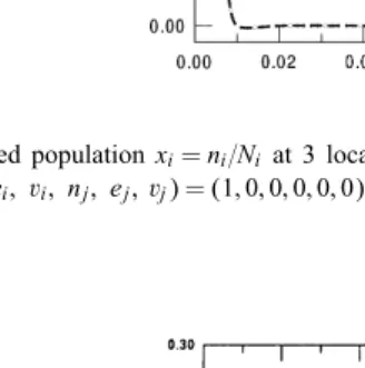
Fig. 3. Normalized population xi=ni=Ni at 3 locationsversusmobilityq, logistic case for set of the model parameters (ni; ei; vi; nj; ej,vj) = (1;0;0;0;0;0):Thenormalizedpopulation at 2 sites is nearly the same, see text.
Fig. 4. Normalized population xi=ni=Ni at 3 locationsversus mobilityq, Penna case for set of the model parameters (ni; ei; vi; nj; ej; vj) = (1;0;0;0;0;0):Thenormalizedpopulation at 2 sites is nearly the same, see text.
critical qc= 0:5B2=(1−B2), and only for B ¡0:5, which yields qc= 0:021. So we
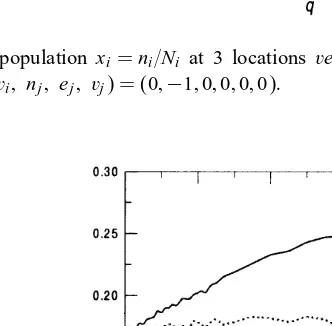
Fig. 5. Normalized population xi=ni=Ni at 3 locationsversus mobilityq, Penna case for set of the model parameters (ni; ei; vi; nj; ej; vj) = (0;−1;0;0;0;0):
Fig. 6. Normalized population xi=ni=Ni at 3 locationsversus mobilityq, Penna case for set of the model parameters (ni; ei; vi; nj; ej; vj) = (0;0;−1;0;0;0):
It should be noted that for still larger q, when migration is forced to become very intensive, the deserted location may become re-occupied again. It may be seen that both logistic and Penna cases (see Fig. 2) are rather similar.
Similar behavior is seen in Figs. 3 and 4 for 3 locations with relative capacities Ni = 1 : 2 : 3. Here, however, the rst two locations (1 : 2) provide nearly the same
normalized population xi at any q and xi tends to zero for intermediate range of q.
Larger q restores x1=x2=x3 at equilibrium.
territories and avoiding densely populated spaces, respectively. This time locations of larger capacities are less densely packed.
We conclude that migration is important and may signicantly alter population distribution.
Acknowledgements
The work was partly supported by grant of Agriculture University in Krakow and also by University of Mining and Metallurgy. Main computer simulations were car-ried out on HP Exemplar S2000 machine at the Academic Computer Center CYFRONET-KRAK OW.
References
[1] D. Brown, P. Rolhery, Models in Biology: Mathematics, Statistics and Computing, Wiley, New York, 1993.
[2] T.J.P. Penna, A bit-string model for biological ageing, J. Stat. Phys. 78 (1995) 1629.
[3] T.J.P. Penna, D. Stauer, Ecient Monte Carlo simulations for biological ageing, Int. J. Mod. Phys. C 6 (1995) 233.
[4] A.T. Bernardes, Monte Carlo simulations of biological ageing, Ann. Rev. Comput. Phys. 4 (1996) 359. [5] S.G.F. Martins, T.J.P. Penna, Computer simulation of sexual selection on age-structured population, Int.