Full Terms & Conditions of access and use can be found at
http://www.tandfonline.com/action/journalInformation?journalCode=ubes20 Download by: [Universitas Maritim Raja Ali Haji], [UNIVERSITAS MARITIM RAJA ALI HAJI
TANJUNGPINANG, KEPULAUAN RIAU] Date: 11 January 2016, At: 20:50
Journal of Business & Economic Statistics
ISSN: 0735-0015 (Print) 1537-2707 (Online) Journal homepage: http://www.tandfonline.com/loi/ubes20
Estimation and Inference for Linear Panel Data
Models Under Misspecification When Both n and T
are Large
Antonio F. Galvao & Kengo Kato
To cite this article: Antonio F. Galvao & Kengo Kato (2014) Estimation and Inference for Linear Panel Data Models Under Misspecification When Both n and T are Large, Journal of Business & Economic Statistics, 32:2, 285-309, DOI: 10.1080/07350015.2013.875473
To link to this article: http://dx.doi.org/10.1080/07350015.2013.875473
Accepted author version posted online: 31 Dec 2013.
Submit your article to this journal
Article views: 256
View related articles
Estimation and Inference for Linear Panel
Data Models Under Misspecification When
Both
n
and
T
are Large
Antonio F. G
ALVAODepartment of Economics, University of Iowa, W284 Pappajohn Business Building, 21 E. Market Street, Iowa City, IA 52242 ([email protected])
Kengo K
ATOGraduate School of Economics, University of Tokyo, 7-3-1 Hongo, Bunkyo-ku, Tokyo 113-0033, Japan ([email protected])
This article considers fixed effects (FE) estimation for linear panel data models under possible model misspecification when both the number of individuals,n, and the number of time periods,T, are large. We first clarify the probability limit of the FE estimator and argue that this probability limit can be regarded as a pseudo-true parameter. We then establish the asymptotic distributional properties of the FE estimator around the pseudo-true parameter whennandTjointly go to infinity. Notably, we show that the FE estimator suffers from the incidental parameters bias of which the top order isO(T−1), and even after the incidental parameters bias is completely removed, the rate of convergence of the FE estimator depends on the degree of model misspecification and is either (nT)−1/2orn−1/2. Second, we establish asymptotically valid inference on the (pseudo-true) parameter. Specifically, we derive the asymptotic properties of the clustered covariance matrix (CCM) estimator and the cross-section bootstrap, and show that they are robust to model misspecification. This establishes a rigorous theoretical ground for the use of the CCM estimator and the cross-section bootstrap when model misspecification and the incidental parameters bias (in the coefficient estimate) are present. We conduct Monte Carlo simulations to evaluate the finite sample performance of the estimators and inference methods, together with a simple application to the unemployment dynamics in the U.S.
KEY WORDS: Cross-section bootstrap; Fixed effects estimator; Incidental parameters problem.
1. INTRODUCTION
It is well known that for a cross-section dataset, the ordi-nary least squares (OLS) estimator is typically consistent for the coefficient vector of the best linear approximation to the conditional mean, even if the conditional mean is not necessar-ily linear (White1980,1982). Such a “robust” nature of OLS is one of the reasons why OLS is popular in empirical studies (Angrist and Pischke2008, Chap. 3).
Suppose now that a panel dataset is available. In such a case, we are typically interested in estimating the partial effects of the observed explanatory variables, xit, on the conditional mean
of the dependent variable,yit, conditional on xit and the
un-observable individual effectci, wherei denotes the index for
individuals andtdenotes the index for time.1For that purpose, a popular strategy is to model the conditional meanE[yit |xit, ci]
as additive in bothciandxit, and linear inxit. The focus is then
on estimating the coefficient vector ofxit. The fixed effect (FE) estimator, which is identical to the OLS estimator treating the individual effects as parameters to be estimated, is often used to estimate the coefficient vector. While for models without strict exogeneity, such as dynamic panel data models, the FE estima-tor is generally inconsistent whenn(the number of individuals) goes to infinity andT (the number of time periods) is fixed
be-1See, e.g., Wooldridge (2001, Chap. 10). We follow the notation used in this reference.
cause of the incidental parameters problem (Neyman and Scott 1948; Nickell1981; Lancaster 2000), it is still a fundamental estimator. In particular, whennandT jointly go to infinity, the FE estimator becomes consistent. Furthermore, after the inci-dental parameters bias is properly corrected, the FE estimator is known to have a centered limiting normal distribution pro-vided thatn/T3
→0, which restrictsT to be mildly large but allowsT to be small relative ton. Such asymptotic properties of the FE estimator under largenandT asymptotics have been extensively studied in the econometrics literature, especially for panel autoregressive (AR) models, partly motivated by the fact that panel datasets with mildly largeT have become available in empirical studies.2
The previous discussion presumes that the model is cor-rectly specified, that is, the conditional mean E[yit|xit, ci]
is truly additive in ci and xit, and linear in xit. The goals
of this article are twofold. The first objective is to study the asymptotic properties of the FE estimator under possible model
2See, e.g., Kiviet (1995), Hahn and Kuersteiner (2002), Alvarez and Arellano (2003), Bun and Carree (2005), Bun and Kiviet (2006), Phillips and Sul (2007), Hansen (2007a), Okui (2008), Okui (2010), and Lee (2012).
© 2014American Statistical Association Journal of Business & Economic Statistics
April 2014, Vol. 32, No. 2 DOI:10.1080/07350015.2013.875473
285
misspecification when bothnandT are large. The asymptotics used is the joint asymptotics where n andT jointly go to
in-finity (more precisely, we indexT bynand letT =Tn→ ∞
asn→ ∞). Assume that{(ci, yi1,xi1, yi2,xi2, . . .)}∞i=1is
inde-pendent and identically distributed (iid), and for eachi≥1, con-ditional onci,{(yit,x′it)′}∞t=1is stationary and weakly dependent.
Suppose thatE[yit |xit, ci] may not be additive inci andxit,
nor linear inxit. Under this setting, we show that the probability limit of the FE estimator is identical to the coefficient vector on xit of the best partiallinear approximation to E[yit |xit, ci],
which gives some rational to use the FE estimator (and its vari-ant) even when the model is possibly misspecified. We regard this probability limit as a pseudo-true parameter (see Section 2for the discussion on interpretation—or plausibility—of this probability limit; especially ifE[yit |xit, ci] is indeed additive
inci andxit, and linear inxit, then the pseudo-true parameter
coincides with the “true” coefficient onxit inE[yit |xit, ci]).
We then establish the asymptotic distributional properties of the
FE estimator around the pseudo-true parameter whennandT
jointly go to infinity. We demonstrate that, as in the correct spec-ification case, the FE estimator suffers from the incidental pa-rameters bias of which the top order isT−1. Moreover, we show that, after the incidental parameters bias is completely removed, the rate of convergence of the FE estimator depends on the de-gree of model misspecification and is either (nT)−1/2orn−1/2.
The second goal of the article is to establish asymptotically valid inference on the (pseudo-true) parameter vector. Since the FE estimator has the bias of orderT−1, the first step is to
re-duce the bias toO(T−2). For that purpose, one can use existing
general-purpose bias reduction methods proposed in the recent nonlinear panel data literature.3For example, one can use the
half-panel jackknife (HPJ) proposed by Dhaene and Jochmans (2009). We refer to Hahn and Kuersteiner (2011) and Arellano and Bonhomme (2009) for alternative approaches on bias cor-rection for FE estimators in panel data models. After the bias is properly reduced, the FE estimator has the centered limiting normal distribution provided thatn/T3→0 orn/T4→0 de-pending on the degree of model misspecification. We are then interested in estimating the covariance matrix or quantiles of the centered limiting normal distribution. To this end, we study the asymptotic properties of the clustered covariance matrix (CCM) estimator (Arellano 1987) and the cross-section boot-strap (Kapetanios2008) under the prescribed setting. We show that the CCM estimator (with an appropriate estimator of the parameter vector) is consistent in a suitable sense and can be used to make asymptotically valid inference on the parameter vector provided thatn/T3
→0 orn/T4
→0. This shows that
inference using the CCM estimator is “robust” to model mis-specification. Also the cross-section bootstrap can consistently estimate the centered limiting distribution of the FE estimator without any knowledge on the degree of model misspecification and hence is robust to model misspecification, and moreover, interestingly,without any growth restriction onT. The second feature of the cross-section bootstrap is notable and shows (in a sense) that the incidental parameters bias does not appear in the bootstrap distribution.
3Hence, there is no new result in the bias correction part.
Allowing for potential model misspecification is of tance in practice. In particular, this article is of practical impor-tance because it provides an interpretation for the FE estimator under potential misspecification, and additionally, it proposes methods for inference in linear panel data model with largen andT that are robust to model misspecification. However, the study of estimation and inference for linear panel data models that are robust to model misspecification is scarce.4An exception is Lee (2012) where he considered the lag order misspecification of panel AR models and established the asymptotic properties of the FE estimator under possible misspecification of the lag order. However, his focus is on the incidental parameters bias and he did not study the inference problem on the pseudo-true parameter. Moreover, Lee (2012) did not cover a general form of model misspecification. This article fills this void. Further-more, the asymptotic properties of the CCM estimator and the cross-section bootstrap when model misspecification and the in-cidental parameters bias (in the coefficient estimate) are present have not been studied in a systematic form and hence is underde-veloped. Hansen (2007b) investigated the asymptotic properties
of the CCM estimator whennandT are large but did not
al-low the case where the incidental parameters bias appears, nor did he cover model misspecification. Kapetanios (2008) studied the asymptotic properties of the cross-section bootstrap when nandT are large, but ruled out the case where the incidental parameters bias appears, nor did he cover model misspecifi-cation as well. Hence, we believe that this article is the first one that establishes a rigorous theoretical ground on the use of the CCM estimator and the cross-section bootstrap when model misspecification and the incidental parameters bias are present. It is important to notice that, even without model misspecifica-tion, these asymptotic properties of the CCM and cross-section bootstrap when the incidental parameters bias is present are new. We conduct Monte Carlo simulations to evaluate the finite sample performance of the estimators and inference methods under misspecification. We are particularly interested in the empirical coverage of the 95% nominal confidence interval. The empirical coverage probability using the CCM and cross-section bootstrap, especially the cross-cross-section bootstrap applied to pivotal statistics, is good. We also apply the procedures dis-cussed in this article to a model of unemployment dynamics at the U.S. state level. The results generate speed of adjustment of the unemployment rate toward the state specific equilibrium of about 17%. In addition, the analysis of estimates indicates that increments in economic growth are associated with smaller unemployment rates.
The organization of this article is as follows. In Section2, we discuss the interpretation of FE estimator under misspeci-fication. In Section3, we present the theoretical results on the asymptotic properties of the FE estimator under misspecifica-tion. In Section4, we present the results on the inference meth-ods. In Section5, we report a Monte Carlo study to assess the finite sample performance of the estimators and inference meth-ods, together with a simple application to a real data. Section6
4Angrist and Pischke (2008, p. 166) remarked that “The set of assumption leading to (5.1.2) is more restrictive than those we used to motivate regression in Chapter 3; we need the linear, additive functional form to make headway on the problem ofunobservedconfounders using panel data with no instruments.”
concludes. We place all the technical proofs to the Appendix. We also include additional theoretical and simulation results in the Appendix.
Notation: For a generic vectorz, letzadenote theath element
ofz. For a generic matrixA, letAabdenote its (a, b)th element.
For a generic vectorzitwith index (i, t), ¯zi =T−1
T
t=1zit. Let
· denote the Euclidean norm. For any matrixA, letAop
denote the operator norm ofA. For any symmetric matrixA, let
λmin(A) denote the minimum eigenvalue ofA. We also use the
notationz⊗2
=z z′for a generic vectorz.
Note on asymptotics: In what follows, we consider the asymp-totic framework in whichT =Tn→ ∞asn→ ∞, so that if we
writen→ ∞, it automatically means thatT → ∞. The limit
is always taken asn→ ∞. This asymptotic scheme is used to capture the situation wherenandT are both large.
2. INTERPRETATION OF FIXED EFFECTS ESTIMATOR UNDER MISSPECIFICATION
In this section, we clarify the probability limit, which we will regard as a pseudo-true parameter, of the FE estimator under the joint asymptotics and discuss interpretation (or plausibility) of the pseudo-true parameter. The discussion is to some extent par-allel to the linear regression case, but there is a subtle difference due to the appearance of individual effects.
Suppose that we have a panel dataset {(ci, yit,xit) :
i=1, . . . , n; t =1, . . . , T}, where ci is an unobservable
individual-specific random variable taking values in an abstract (Polish) space,yitis a scalar-dependent variable andxitis a
vec-tor ofpexplanatory variables. Typically, the random variableci,
which is constant over time, represents an individual character-istic such as ability or firm’s managerial quality which we would include in the analysis if it were observable (see Wooldridge 2001, Chap. 10). Assume that{(ci, yi1,xi1, . . . , yiT,xiT)}ni=1
is iid, and for each 1≤i≤n, conditional onci,{(yit,x′it)′} T t=1
is a realization of a stationary weakly dependent process.5 Here, the marginal distribution of (ci, yit,xit) is invariant with
respect to (i, t). Typically, we are interested in estimating the partial effects of xit on the conditional mean E[yit |xit, ci]
with keeping ci fixed. A “standard” linear panel data model
assumes that the conditional mean is of the formg(ci)+x′itβ
with unknown function g and vector β, and redefines ci by
g(ci) since, in any case, ci is unobservable and modeling a
functional form for the individual effect is virtually meaningless (see Angrist and Pischke 2008, Chap. 5). In this article, the “correct” specification refers to that the conditional mean
E[yit |xit, ci] is written in the formg(ci)+x′itβ, and “model
misspecification” signifies any violation of this condition. For instance, this can happen if there are omitted variables or if nonlinearity occurs in the model. We discuss more details below (see Examples 1 and 2 below for concrete examples).
5That is, the data are iid across individuals, but for each individual, conditional on the individual effect, the data are (weakly) dependent across time.
The FE estimator defined by
β=
is consistent for the coefficient vector onxitasngoes to infinity andT is fixed if the specification is correct (for the moment, assuming thatβ exists) and additionally the strict exogoneity assumptionE[yit| xi1, . . . ,xiT, ci]=E[yit|xit, ci] is met. If
the strict exogoneity assumption is violated, then the FE esti-mator is not fixed-T consistent, but asT → ∞withn, the FE estimator becomes consistent for the coefficient vector on xit
provided that the specification is correct. Suppose now that the specification is not correct, that is, E[yit |xit, ci] may not be
written in the form g(ci)+x′itβ, and consider the probability
limit of the FE estimator when nandT jointly go to infinity. Proposition 1 ahead shows that, subject to some technical
con-ditions, we have, asn→ ∞andT =Tn→ ∞,
moment, assume that some moments exist). To gain some in-sight, we provide a heuristic derivation of this probability limit
under the sequential asymptotics whereT → ∞first and then
n→ ∞. By definition, we have
t=1 is weakly dependent conditional on
ci, as T → ∞ first, we have T−1
In what follows, we discuss an interpretation ofβ0defined in
(2.2). A direct interpretation is thatβ0is the coefficient vector of
the best linear approximation toE[yit |xit], but this
interpreta-tion does not explain the connecinterpreta-tion with the primal object of es-timating the partial effects ofxitonE[yit| xit, ci]. However, the
and hence β0 is the coefficient vector on xit of the best
par-tial linear predictor. Moreover, it is not difficult to see that
g0(ci)+x′itb0 is indeed the best partial linear approximation
toE[yit |xit, ci], that is,
E[(E[yit| xit, ci]−g0(ci)−x′itb0)2]
= min
g∈L2(c1),b∈Rp
E[(E[yit |xit, ci]−g(ci)−x′itb) 2
]. (2.3)
Therefore, the vector β0 defined by (2.2) is identical to the
coefficient vector onxitof the best partial linear approximation
toE[yit |xit, ci] in (2.3). Just as the coefficient vector of the
best linear approximation to the conditional mean is a parameter of interest in the cross-section case, as discussed in Chapter 3 of Angrist and Pischke (2008), the vectorβ0here can be regarded
as a plausible parameter of interest in the panel data case. Hence, in this article, we considerβ0to be a parameter of interest and
treatβ0as a pseudo-true parameter.
Remark 1. Clearly ifE[yit |xit, ci] is indeed additive in ci
and xit, and linear in xit, then β0 coincides with the “true”
coefficient onxitinE[yit |xit, ci].
As in the cross-section case, letting the approximation er-ror denoteǫit =yit−g0(ci)−x′itβ0 =yit−x′itβ0, we have a
regression form
yit=g0(ci)+x′itβ0+ǫit, E[ǫit |ci]=0, E[xitǫit]=0.
(2.4)
Importantly, the “error term”ǫithere may not satisfy the
condi-tional mean restrictionE[ǫit| xit, ci]=0 due to possible model
misspecification.
In (2.4), there are two scenarios on violation of the condi-tional mean restrictionE[ǫit |xit, ci]=0. One is the case where
E[ǫit|xit, ci]=0 with positive probability butE[xitǫit|ci]= 0a.s. The other is the case whereE[xitǫit|ci]=0with
posi-tive probability. Depending on these two cases, the asymptotic properties of the FE estimatordochange drastically (see Sec-tion 3). Generally, both cases can happen. We give three simple examples to fix the idea.
Example 1. Panel AR model with misspecified lag order. Suppose that the true data-generating process follows a panel AR(2) model
yit =ci+φ1yi,t−1+φ2yi,t−2+uit, ci⊥⊥{uit}t∈Z,
ci ∈R, {uit}: iid, E[uit]=0,
where (φ1, φ2) is such thatφ2+φ1<1, φ2−φ1<1 and−1<
φ2<1. Conditional onci,{yit}t∈Z is stationary and typically
weakly dependent. By a simple calculation, we have E[yit |
ci]=ci/(1−φ1−φ2). Lettingyit =yit−E[yit |ci], we have
yit=φ1yi,t−1+φ2yi,t−2+uit. Hence,{yit}t∈Z is independent
ofci. Suppose now that we incorrectly fit a panel AR(1) model.
Note that in this case, we have
E[yit|yi,t−1, ci]=ci+φ1yi,t−1+φ2E[yi,t−2|yi,t−1, ci].
Hence,E[yit|yi,t−1, ci] is generally a nonlinear function of
ci and yi,t−1 except for the cases where φ2=0 or the
dis-tribution of uit is normal. Here, the solution of the equation
E[yi,t−1(yit−β0yi,t−1)]=0 is the first-order autocorrelation
coefficient of {yit}, that is, β0=cov(yit,yi,t−1)/Var(yi,t−1).
Lettingǫit =yit−β0yi,t−1=(φ1−β0)yi,t−1+φ2yi,t−2+uit,
we haveyit =β0yi,t−1+ǫit, that is,yit=(1−β0)ci/(1−φ1−
φ2)+β0yi,t−1+ǫit. By the independence of{yit}fromci, we
haveE[yi,t−1ǫit|ci]=E[yi,t−1ǫit]=0 a.s. Lee (2012) studied
such panel AR models with misspecified lag order in detail. This article covers lag order misspecification as a special case.
Example 2. Static panel with a mismeasured regressor. Sup-pose the true data-generating process is as follows:
yit =ci+φxit∗ +uit, ci ∈R, E[uit |xit∗, ci]=0.
In addition,
xit =xit∗ +vit, E[vit |x∗it, ci]=0.
Suppose thatci, uit, andvitare independent, and we incorrectly
fit a model usingxitinstead ofxit∗. Here, we have
xit=xit−E[xit|ci]=xit∗ +vit−E[xit∗ |ci]=xit∗ +vit,
where x∗
it=xit∗ −E[xit∗ |ci], and yit =yit−E[yit |ci]=
φx∗
it+uit. Hence, the solution to the equation E[xit(yit−
βxit)]=0 is given by
β0=E
xit2 −1E[yitxit]=
E[(x∗ it)
2]
E[(x∗ it)2]+E
v2 it
φ.
Finally, byǫit=yit−β0xit, we haveE[xitǫit |ci]=E[(xit∗) 2
|
ci]φ−(E[(xit∗) 2
|ci]+E[v2it])β0, which is generally non-zero.
Example 3. Random coefficients AR model. Suppose that the true data-generating process follows the following random coefficients AR(1) model:
yit =ciyi,t−1+uit, ci⊥⊥{uit}t∈Z, |ci|<1, uit ∼N(0,1),iid
In this case,E[yit |yi,t−1, ci]=ciyi,t−1. It is routine to verify
that
yit|ci ∼N
0,1/1−ci2.
Suppose that we incorrectly fit a panel AR(1) model. Here, yit =yit−E[yit |ci]=yit and the solution of the equation
E[yi,t−1(yit−β0yi,t−1)]=0 is given by
β0=
Eciyi,t2−1
Ey2 i,t−1
= E
ci/
1−c2
i
E1/1−c2 i
.
Here,ǫit=yit−β0yi,t−1, and
E[yi,t−1ǫit|ci]=E
ciyi,t2−1−β0yi,t2−1|ci =
ci−β0
1−c2 i
,
which is nonzero a.s. ifciobeys a continuous distribution.
Remark 2 (Interpretation under pseudo-likelihood
setting). The results in this article could be interpreted
as corresponding to the pseudo-likelihood model. Under the additional assumptions of independence and normality, the resulting (conditional) maximum likelihood estimator (MLE) ofβ(givenc1, . . . , cn) is identical to the FE estimator. Thus, the
FE estimator defined in (2.1) can be viewed as a pseudo-MLE.
Remark 3(Discussion on Lu, Goldberg, and Fine2012). Lu,
Goldberg, and Fine (2012) made an interesting observation
about the pseudo-true parameter when the link function is mis-specified for the generalized linear model (see their Corollary 1). That is, the pseudo-true parameter is proportional to the true one up to nonzero scalar. However, their setting is significantly different from ours; first of all in Corollary 1 they assumed that
the true model satisfies a generalized linear model but only the link function is misspecified, and only cross-section data are available. In our case basically no “model” is assumed (and hence the “true parameter” is not well-defined in general), so that their result does not extend to our setting.
Remark 4(Alternative estimators). In this article, we focus on the FE estimator. This is because the FE estimator is widely used in practice and, as we have shown, the probability limit of the FE estimator under misspecification admits a natural and plausible interpretation, parallel to the linear regression case. There could be alternative estimators; for example, we could consider the av-erage of the individualwise OLS estimators, that is, letβidenote the OLS estimator obtained by regressingyit on (1,x′it)′ with
each fixed i, and consider the estimatorβave=n−1n i=1βi.
However, this estimator does not share the interpretation that the FE estimator possesses. In some cases, the probability limit ofβavehappens to be identical toβ0, but not in general. To keep
tight focus, we only consider the FE estimator in what follows.
3. ASYMPTOTIC PROPERTIES OF FIXED EFFECTS ESTIMATOR UNDER MISSPECIFICATION
In this section, we study the asymptotic properties of the FE estimator under possible model misspecification (i.e., E[yit | xit, ci] is not assumed to be additive inciandxit, nor linear in xit). We make the following regularity conditions.
(A.1) (ci, yit,xit)∈S×R×Rp, whereSis a Polish space.
{(ci, yi1,xi1, yi2,xi2, . . .)}∞i=1is iid, and for eachi≥1,
conditional onci,{(yit,xit′ )′}∞t=1is a stationaryα-mixing
process with mixing coefficientsα(k|ci). Assume that
there exists a sequence of constantsα(k) such thatα(k| ci)≤α(k) a.s. for allk≥1, and
∞ k=1kα(k)
δ/(8+δ) <
∞for someδ >0.
(A.2) Define yit=yit−E[yit|ci] and xit =xit−E[xit |
ci] (assume thatE[yit |ci] andE[xit|ci] exist). There
exists a constantM >0 such thatE[|yit|8+δ|ci]≤M
a.s. andE[xit8+δ
|ci]≤Ma.s., whereδ >0 is given
in (A1).
(A.3) Define the matrixA=E[xitx′it]. Assume that the
ma-trixAis nonsingular.
In condition (A1),ci is an unobservable, individual-specific
random variable allowed to be dependent withxit in an arbi-trary form. Condition (A1) assumes that the observations are independent in the cross-section dimension, but allows for de-pendence in the time dimension conditional on individual ef-fects. We refer to Section 2.6 of Fan and Yao (2003) for some basic properties of mixing processes. Condition (A1) is simi-lar to Condition 1 of Hahn and Kuersteiner (2011) and allows for a flexible time series dependence. The mixing condition is also similar to Assumption 1 (iii) of Gonc¸alves (2011), while she allowed for cross-section dependence. The mixing condi-tion is used only to bound covariances and moments of sums of random variables, and not crucial for the central limit theo-rem. Therefore, in principle, it could be replaced by assuming directly such bounds. We assume the mixing condition to make the article clear. Note that because of stationarity assumption
made in (A1), the marginal distribution of (ci, yit,xit) is
invari-ant with respect to (i, t), that is, (ci, yit,xit) d
=(c1, y1,1,x1,1).6
The stationary assumption rules out time trends, but is needed to well define the pseudo-true parameterβ0, and maintained in
this article. Extensions to nonstationary cases will need differ-ent analyses and are not covered in this article. Condition (A2) is a moment condition. As usual, there is a trade-off between the mixing condition and the moment condition. Condition (A2) implies thatE[|ǫit|8+δ|ci]≤M′a.s. for some constantM′>0.
Condition (A3) is a standard full rank condition. Ifxitcontains an element that does not vary over time for anyi, then the cor-responding element ofxit is equal to zero for allt, and in this case, condition (A3) could not be satisfied. Thus, (A3) excludes the analysis of time-constant variables.
Now we introduce some notation. Recall the FE estimator:
β =
1
nT
n
i=1 T
t=1
(xit−x¯i)(xit−x¯i)′ −1
×
1
nT
n
i=1 T
t=1
(xit−x¯i)(yit−y¯i)
=:A−1S, (3.1)
where A=(nT)−1n i=1
T
t=1(xit−x¯i)(xit−x¯i)′ and S=
(nT)−1n i=1
T
t=1(xit−x¯i)(yit−y¯i). Under conditions (A1)–
(A3), the matrixAon the right side is nonsingular with proba-bility approaching one (see Lemma C.1 in AppendixC).
Recall thatβ0is defined by (2.2) andǫitis defined byǫit=
yit−x′itβ0(see the previous section). Define
BT =
|k|≤T−1
1−|k|
T
E[x1,1ǫ1,1+k],
DT =
|k|≤T−1
1−|Tk|
E[x1,1x′
1,1+k].
Here and in what follows, for the notational convenience, terms likeE[x1,1ǫ1,1+k] fork <0 are understood asE[x1,1−kǫ1,1], that
is,
E[x1,1ǫ1,1+k] :=E[x1,1−kǫ1,1], k <0.
We shall obey the same convention to other such terms. For ex-ample,E[x1,1x′1,1+k] :=E[x1,1−kx′1,1] fork <0. We first note
that under conditions (A1)–(A3), bothBT andDT are well
be-haved in the following sense.
Lemma 1. Under conditions (A1)–(A3), we have ∞k=−∞ |k|E[x1,1ǫ1,1+k]<∞and
∞
k=−∞E[x1,1x′1,1+k]op<∞.
All the technical proofs for Section 2 are gathered in AppendixC.
6The stationarity assumption means that for dynamic models, the initial condi-tion,yi0, is drawn from the stationary distribution, conditional onci.
We now state the asymptotic properties of the FE estimator.
Proposition 1. Suppose that conditions (A1)–(A3) are
satis-fied. LettingT =Tn→ ∞asn→ ∞, we have
We stress that Proposition 1 holds without any specific growth condition on T. Also note that this proposition implies that
β→P β0as long asT =Tn→ ∞.
We discuss some implications of Proposition 1. First, Propo-sition 1 shows that the FE estimator has the bias term of the form
which, following the literature, we call the “incidental parame-ters bias.” There are two sources that contribute to the incidental parameters bias. The main source is conditional correlation be-tweenxisandǫitfors=tconditional onci, which arises from
using ¯xiinstead ofE[xi1 |ci] inS. Another source, which only
contributes to higher order terms, is conditional correlation be-tweenxisandxitfors=tconditional onci, which arises from
using ¯xi instead ofE[xi1|ci] inA. Proposition 1 makes
ex-plicit the incidental parameters bias of any order, which appears to be new even in the correct specification case (but under the current set of assumptions).7The expansion (3.2) is important
7Dhaene and Jochmans (2010) considered higher order bias corrections for the panel AR model with exogenous variables, fixed effects, and unrestricted initial observations. The assumptions behind their article are different from ours: here more general models (not restricted to panel AR models, and allowing for
in investigating the asymptotic properties of the cross-section bootstrap in Section 4.
Second, Proposition 1 shows that, aside from the incidental parameters bias, the rate of convergence of the FE estimator depends on the degree of model misspecification, that is, after the incidental parameters bias is completely removed, the FE estimator is√nT-consistent ifE[xitǫit|ci]=0a.s. and √n
-consistent otherwise. In fact, the rate of convergence of the FE estimator (after the incidental parameters bias is removed) depends on the order of the covariance matrix of the term
1
}. On the other hand, the second term is zero if E[xitǫit |ci]=0 a.s., but ≍n−1 otherwise, which
shows that nT =O{(nT)−1} if E[xitǫit |ci]=0 a.s. and
nTop≍n−1otherwise. Intuitively, unlessE[xitǫit|ci]=0
a.s.,xitǫit is unconditionally equicorrelated across t, so that
nT has the slow raten−1(ifE[xitǫit |ci]=0a.s., by
condi-tion (A1), the covariance betweenxisǫisandxitǫitconverges to
zero sufficiently fast as|s−t| → ∞, sonT has the faster rate
(nT)−1).
In some cases, at least theoretically, it may happen that
E[xitǫit|ci]=0with positive probability but for some nonzero r ∈Rp
,r′A−1
E[xitǫit|ci]=0 a.s., which corresponds to the
case where the matrixE[E[x1,1ǫ1,1 |c1]⊗2] is nonzero but
de-generate. In such a case, we have the expansion
r′
model misspecification) are covered, but Dhaene and Jochmans (2010) covered nonstationary cases.
where the leading term of the right side multiplied by √
nT is asymptotically normal with mean zero and variance
limn→∞[(nTn)r′A−1nTnA− 1r]<
∞. This shows that, after subtracting the incidental parameters bias, the FE estimator may have different rates of convergence within its linear combina-tions. Moreover, the remainder term in the expansion (3.4) has the constant term of ordern−1, so that the extra bias term of ordern−1appears in such a case.8By this, if additionallyT /n
goes to some positive constant, the limiting normal distribution of the right side on (3.4) multiplied by√nT has a nonzero bias in the mean of which the size is proportional to√T /n. However, such a case seems to be rather exceptional and we mainly focus on the case, where the matrixis always nonsingular (i.e.,
is nonsingular in either case ofE[xitǫit |ci]=0a.s. or not).
It is possible to have an alternative expression of the bias term of orderT−1.
Corollary 1. Suppose that conditions (A1)–(A3) are satisfied. Then, we have
BT =∞k=−∞E[x1,1ǫ1,1+k]+O(T−1)=:B+O(T−1).
In particular, the bias term of orderT−1in the expansion (3.2)
is rewritten asT−1A−1B.
Finally, we provide some comments on the relation to the previous work.
Remark 5(Relation with Lee2012). Proposition 1 is a non-trivial extension of Theorem 2 of Lee (2012), in which he estab-lished the asymptotic properties of the FE estimator for panel AR models with exogenous variables allowing for lag order misspecification. Proposition 1 allows for a more general form of model misspecification, including lag order misspecification as a special case, and exhausts the incidental parameters bias of any order.
Remark 6 (Relation with Hansen 2007b). Proposition 1 is related to Hansen (2007b). Hansen (2007b) considered a model yit =x′itβ0+ǫit withE[ǫit|xi1, . . . ,xiT]=0 for all
1≤t≤T orE[xitǫit]=0, and showed that the OLS estimator
is√n-consistent if there is no condition on time series depen-dence and √nT-consistent if a mixing condition is satisfied for time series dependence. What matters for the rate of con-vergence of the OLS estimator in Hansen (2007b) is the order of the covariance matrix of the term (nT)−1ni=1
T
t=1xitǫit,
which is O(n−1) in the “no mixing” case and O{(nT)−1} in the mixing case. While there is a similarity, Proposition 1 is not nested to his results in several aspects. First, in Proposition 1, the rate of convergence of the FE estimator (after the incidental pa-rameters bias is removed) depends on the degree of model mis-specification (i.e.,E[xitǫit |ci]=0a.s. or not), rather than the
assumption on time series dependence. Second, while his model covers panel data models with individual effects by consider-ing (yit,x′it)′ to be transformed variables (yit−y¯i,x′it−x¯′i)′,
the mixing assumption is not satisfied for the transformed vari-ables as he admitted in footnote 3, so that his Theorem 3 does not apply to models with individual effects. Additionally, his
8By the proof of Proposition 1, it is shown that the remainder term in the expansion (3.4) is in fact further expanded as−n−1r′A−1
E[E[x1,1x′ 1,1| c1]A−1E[x1,1ǫ1′,1|c1]]+OP[n−1/2max{n−1, T−1}].
Assumption 3 essentially requires thatE[xisǫit |ci]=0for all
1≤s, t ≤T under our setting (if we think of (yit,x′it)′as
trans-formed variables (yit−y¯i,x′it−x¯′i)′), so that his results do not
cover the case where the incidental parameters bias appears. On the other hand, while we exclusively assume that{(yit,x′it)′}∞t=1
is mixing conditional onci, Hansen (2007b) covered the case
where no such mixing condition is satisfied. Therefore, the two papers are complementary in nature.
Remark 7(Relation with Arellano and Hahn2006). Arellano and Hahn (2006) obtained a general incidental parameters bias formula for nonlinear panel data models, allowing for potential
model misspecification, whenn/T is going to some constant.
Their general result could be applied to the present setting in the case whereE[xitǫit |ci]=0. However, the stochastic
ex-pansion (3.2) is not derived in Arellano and Hahn (2006); (3.2) exhausts the incidental parameters bias up to infinite order, and covers the case whereE[xitǫit|ci]=0. This expansion is also
the key for studying the properties of cross-section bootstrap.
4. INFERENCE
4.1 Bias Correction
By Proposition 1, the FE estimator has the bias of orderT−1. In many econometric applications,Tis typically smaller thann, so that the normal approximation neglecting the bias may not be accurate in either case ofE[xitǫit|ci]=0orE[xitǫit |ci]=0.
Therefore, the first step to make inference onβ0is to remove
the bias of orderT−1and reduce the order of the bias toT−2.
Under model misspecification, bias reduction methods that de-pend on specific models (such as panel AR models) may not work properly. Instead, we can use general-purpose bias reduc-tion methods proposed in the recent nonlinear panel data lit-erature. For example, the half-panel jackknife (HPJ) proposed by Dhaene and Jochmans (2009) is able to remove the bias of orderT−1even under model misspecification. Suppose thatTis even. LetS1= {1, . . . , T /2}andS2= {T /2+1, . . . , T}. For
l=1,2, construct the FE estimatorβS
l based on the split
sam-ple {(yit,x′it)′:i=1, . . . , n;t ∈Sl}. Then, the HPJ estimator
is defined byβ1/2=2β−(βS
1+βS2)/2. Using the expansion
(3.2) and Corollary 1, asT =Tn→ ∞, we have the expansion
β1/2−β0+O(T−2)
=A−1
1
nT
n
i=1 T
t=1
xitǫit
+OPn−1/2maxdnT−1/2, T−1 ,
(4.1)
so that the bias is reduced to O(T−2) in either case.
There-fore, we have √dnT(β1/2−β0) d
→N(0, A−1A−1) provided
that √dnT/T2→0. Dhaene and Jochmans (2009) proposed
other automatic bias reduction methods applicable to general nonlinear panel data models. Their bias reduction methods are basically applicable to the model misspecification case.9
9For example, the higher order bias correction methods proposed in Dhaene and Jochmans (2009) could be adapted here; such higher order bias correction would be a good option whenn/T is large.
Alternatively, a direct approach to bias correction is to analyt-ically estimate the bias term. In this case, we typanalyt-ically estimate the first-order bias term−A−1Bby using the technique of HAC
covariance matrix estimation (see Hahn and Kuersteiner2011). Moreover, another alternative approach is to use bias reduc-ing priors on individual effects (see, e.g., Arellano and
Bon-homme 2009, and references therein). See also Arellano and
Hahn (2007) for a review on bias correction for FE estimators in nonlinear panel data models.
4.2 Clustered Covariance Matrix Estimator
By the previous discussion, a bias-corrected estimatorβ typ-ically has the expansion
β−β0+O(T−2)
=A−1
1
nT
n
i=1 T
t=1
xitǫit
+OPn−1/2maxdnT−1/2, T−1 .
(4.2)
Given this expansion, provided that √dnT/T2→0, the
dis-tribution of β can be approximated by N(β0, A−1nTA−1).
Statistical inference on β0 can be implemented by using this
normal approximation. As usual, since the matricesAandnT
are unknown, we have to replace them by suitable estimators. A natural estimator ofAisAdefined in (3.1), which is in fact con-sistent (i.e.,A→P A) as long asT =Tn→ ∞(see Lemma C.1
in AppendixC). We thus focus on the problem of estimating the matrixnT. We consider the estimator suggested by Arellano
(1987):
nT =
1
n2 n
i=1
1
T
T
t=1
(xit−x¯i)ǫit
⊗2
,
whereǫit =yit−y¯i−(xit−x¯i)′βandβis a suitable
estima-tor ofβ0. Proposition 2 establishes the rate of convergence of
nT. All the technical proofs of this section are gathered in
AppendixD.
Proposition 2. Suppose that conditions (A1)–(A3) are sat-isfied. Let β be any estimator of β0 such that β−β0 =
OP[max{dnT−1/2, T−1}]. Letting T =Tn→ ∞ as n→ ∞, we
have
nT =nT +OP
maxn−1/2T−1dnT−1/2, n−1/2dnT−1 .
In particular, as long as T =Tn→ ∞, we have nT −
nTop=oP(dnT−1).
Remark 8(Initial estimators). In Proposition 2,βcan be the FE estimator. Actually, using a bias-corrected estimator instead does not change the rate of convergence ofnT. However, in the
case whereTis relatively small, the FE estimator can be severely biased, which may affect the finite sample performance ofnT.
Thus, it is generally recommended to use a bias-corrected esti-mator ofβ0in the construction ofnT.
Remark 9 (Relation with Hansen 2007b). The results of Hansen (2007b) are not directly applicable to the asymptotic properties of nT described in Proposition 2. This is because
the individual dummies that control for FEs are not included
in the model of (Hansen2007b, see also previous Remark 6). Thus, in contrast with Hansen (2007b),√ndnT(nT −nT) is
not asymptotically normal with mean zero unless√dnT/T →0.
The main reason is thatnT has a bias of ordern−1/2T−1d− 1/2 nT
due to using ¯xi instead ofE[xi1|ci]. This bias appears even
if we could use ǫit in place ofǫit. However, for inference
purposes, the rate of convergence given in Proposition 2 is suf-ficient, and we do not consider the bias correction tonT.
Assume now that is nonsingular in either case of
E[xitǫit|ci]=0a.s. or not. Consider testing the null hypothesis
H0:Rβ0=r, whereRis aq×pmatrix with rankq(q ≤p),
andr∈Rq is a constant vector. Suppose that we have a
bias-corrected estimatorβhaving the expansion (4.2). Then under the null hypothesis, thet-type (forq =1) and Wald-type statistics
t = Rβ−r
RA−1
nTA−1R′
(q =1) and
F =(Rβ−r)′[RA−1nTA−1R′]−1(Rβ−r), (4.3)
converge in distribution to N(0,1) and χ2
q, respectively,
pro-vided that √dnT/T2→0. For example, for q =1, provided
that√dnT/T2→0,
t =
√
dnT(Rβ−r)
RA−1(d
nTnT)A−1R′
= √
dnT(Rβ−r)
√
RA−1A−1R′(1+oP(1)) d
→N(0,1),
where the second equality is because A=A+oP(1) and
dnTnT =dnTnT +oP(1)=+oP(1). The same machinery
applies to the Wald-type statistic. Importantly, in the construc-tion oft-type or Wald-type statistics, we do not need any knowl-edge on the degree of model misspecification.
The resulting estimatorA−1nTA−1of the covariance matrix
A−1nTA−1is often called the CCM estimator in the literature.
The CCM estimator is popular in empirical studies. The appeal-ing point of the CCM estimator, as discussed in Hansen (2007b), is the fact that it is free from any user-chosen parameter such as a bandwidth. The previous discussion shows that inference using a suitable bias-corrected estimator and the CCM estimator is “robust” to model misspecification.
4.3 Cross-Section Bootstrap
Bootstrap is generally used as a way to estimate the distribu-tion of a statistic (see Horowitz2001, for a general reference on bootstrap). For panel data, how to implement bootstrap is not necessarily apparent. See Kapetanios (2008) for some pos-sibilities in bootstrap resamplings for panel data. We here study, among them, the cross-section bootstrap.
Let zi =(z′
i1, . . . ,z′iT)′ with zit=(yit,x′it)′. The
cross-section bootstrap randomly drawsz∗
1, . . . ,z∗nfrom{z1, . . . ,zn}
with replacement. The bootstrap FE estimator β∗ is defined byβ in (2.1) with z1, . . . ,zn replaced by z∗
1, . . . ,z∗n. By this
definition, we can expressβ∗as
where wni is the number of times that zi is “redrawn” from
{z1, . . . ,zn}. The vector (wn1, . . . , wnn)′ is independent of
{ci,zit :i≥1, t≥1}and multinomially distributed with
pa-rametersnand (probabilities)n−1, . . . , n−1.
We need to prepare some notation and terminology. LetPW
denote the probability measure with respect town1, . . . , wnn.
We are now in position to state the main result of this section.
Proposition 3. Suppose that conditions (A1)–(A3) are
satis-fied. LettingT =Tn→ ∞asn→ ∞, we have in probability. Therefore, provided that is nonsingular, we have where the inequalities are interpreted coordinatewise.
Interestingly, Proposition 3 shows that despite the fact that the original FE estimator has the incidental parameters bias of which the top order isT−1, as shown in Proposition 1, the
boot-strap distribution made by applying the cross-section bootboot-strap to the FE estimator does not have the incidental parameters bias. As a consequence, the bootstrap distribution approach-ing the centered normal distribution holds without any specific growth condition onT. In fact, this is not surprising. The main source of the incidental parameters bias comes from the term
n−1ni=1x¯˜iǫ¯i, which is linear in the cross-section dimension.
The bootstrap analogue of this term is thusn−1ni=1wnix¯˜iǫ¯i,
so that the difference of these terms has mean zero with respect toPW. The same machinery applies to the termn−1
n i=1x¯˜ix¯˜′i,
so that the incidental parameters bias is completely removed in the bootstrap distribution.
The previous discussion also has the following implication: the cross-section bootstrap cannot be used as a way to correct the incidental parameter bias. Recall that in the cross-section case, the bootstrap can be used to correct the second-order bias coming from the quadratic term; here, the incidental parameters bias comes from the terms linear in the cross-section dimension, so that the cross-section bootstrap does not work as a way to correct the bias.
where (·) is the distribution function of the standard normal distribution (recall thatza is theath element of a vectorzand
Aabdenotes the (a, b)-element of a matrixA). Suppose that we have a bias-corrected estimatorβ having the expansion (4.2). Then by a standard argument, we can deduce that
Pβ0a≤βa+q(α)=α+o(1),
provided that√dnT/T2→0. Note thatq(α) can be computed
with any precision by using simulation. Moreover, the compu-tation ofq(α) does not require any knowledge on the speed of
dnT, and in this sense the cross-section bootstrap is robust to
model misspecification.
An analogous result holds for the HPJ estimator (see Sec-tion 4.1).
Corollary 2. Suppose that conditions (A1)–(A3) are satisfied. Letβ∗1/2denote the HPJ estimator based on the bootstrap sample {z∗
in probability. Therefore, provided that is nonsingular, we have
This corollary follows directly from the definition of the HPJ estimator and Proposition 3, and hence we omit the proof. Ba-sically, the conclusion of Corollary 2 holds for other reasonable bias-corrected estimators. We do not attempt to encompass gen-erality in this direction.
Analogous results hold for pivotal statistics. Because of the space limitation, we push the formal results on pivotal statistics to AppendixA.
Remark 10(Higher order properties). The higher order prop-erties of the cross-section bootstrap will be very complicated in this setting and we do not attempt to study them here. However,
it is of interest to quantify the order of the convergence in, say, (A.1), which is left to future research.
Remark 11 (Relation to the previous literature). There are some earlier works on the bootstrap for panel data. Bertrand, Duflo, and Mullainathan (2004) called the cross-section boot-strap in this article the “block bootboot-strap” and studied its nu-merical properties by using simulations, but did not study its theoretical properties. Kapetanios (2008) developed the asymp-totic properties of the cross-section bootstrap when the strict exogeneity is met, hence excluding the possibility that the in-cidental parameters bias appears. Gonc¸alves (2011) studied the asymptotic properties of the moving block bootstrap for panel data, which resamples the data in the time series dimension and hence is different from the cross-section bootstrap. Impor-tantly, while Gonc¸alves (2011) allowed for cross-section de-pendence which we exclude here, she assumed that the number of time periods, T, is sufficiently large (typicallyn/T →0) so that the incidental parameters bias does not appear. Finally, Dhaene and Jochmans (2009) proposed to use the cross-section bootstrap for inference for nonlinear panel data models such as panel probit models, but did not give any theoretical result. The asymptotic properties of the cross-section bootstrap were largely unknown when the incidental parameters bias appears, even without model misspecification, and the results in this sec-tion contribute to filling this void and give useful suggessec-tions to empirical studies.
Remark 12 (Weighted bootstrap). In (4.4), the weights
wn1, . . . , wnnare multinomially distributed. It is possible to
con-sider other weights. A perhaps simplest variation is to draw inde-pendent weightsw1, . . . , wnfrom a common distribution with
mean 1 and variancev >0, which corresponds to theweighted bootstrap (see, e.g., Ma and Kosorok 2005). Let βW denote (4.4) withwnireplaced by these independent weightswi. Then,
the conclusion of Proposition 3 holds withβ∗ replaced byβW and√dnT replaced by√dnT/v. Since the proof is completely
analogous, we omit the details for brevity.
Remark 13(Covariance matrix estimation). So far, we have discussed the distributional properties of the cross-section boot-strap. Given Proposition 3, it is natural to estimate the asymp-totic covariance matrixA−1
nTA−1by the conditional
covari-ance matrix ofβ∗−β. However, since convergence in distri-bution does not imply moment convergence, Proposition 3 does not guarantee that dnTEPW[(β
∗−β)(β∗−β)′]→A−1A−1
in probability. See Shao (1992) for some examples of incon-sistency of bootstrap variance estimators. In linear regression models with pure cross section or time series data, Gonc¸alves and White (2005) discussed bootstrap-based covariance matrix estimation. In Gonc¸alves and White (2005), they made a modi-fication to the bootstrap least-square estimator, to guarantee the bootstrap estimator to satisfy a uniform integrability condition. Their modification is a sort of “trimming” to the second mo-ment matrix. By doing so, they established the consistency of the bootstrap covariance matrix estimator. In the present panel data case, while their modification is straightforward to adapt to the FE estimator, it is not clear whether it actually works at the proof level. In Proposition 3, what we have done are:
(i) to implement higher order stochastic expansions to the FE estimator to exhaust the incidental parameters bias of any order; (ii) to implement (i) to the bootstrap analogue; (iii) to elimi-nate the incidental parameters bias by taking the difference. In step (ii), we need expansions ofA∗, or more precisely (A∗)−1
. Simply bounding (A∗)−1op from above, as Gonc¸alves and
White (2005) did in Step 3 of the proof of their Theorem 1, will leave the bias in the bootstrap distribution and cause a problem in establishing uniform integrability. We leave this as an open problem.
5. NUMERICAL EXAMPLES
In this section, numerical examples to illustrate the methods discussed in this article are provided. Both Monte Carlo exper-iments and a real data analysis are presented. All the numerical experiments were performed on the statistical software R (R
De-velopment Core Team2008). Computer programs to replicate
the numerical analyses are available from the authors.
5.1 Simulation Experiments
We use several different designs of simulation experiments to assess the finite sample performance of the estimates and inference procedures discussed in the previous sections. In the first design, as a benchmark, we analyze the estimates and in-ference procedures under correct specification. The true data-generating process (DGP) in the first design follows a panel AR(1) model and we (correctly) fit panel AR(1). The next four models are designed to study the estimates and inference pro-cedures under misspecification.10In the second design, the true
DGP follows a panel AR(2) model (see Example 1 in Section 2); in the third design, we extend the true AR(2) DGP and in-clude two lags of exogenous regressors; and in the last design, the true DGP follows a random coefficient AR(1) model (see Example 2 in Section2). In each of these cases, we incorrectly fit a panel AR(1) model and estimate the slope parameter. Note that the first three cases correspond to “E[xitǫit|ci]=0” case
and the last case corresponds to “E[xitǫit|ci]=0” case. The
following sample sizes are considered:n∈ {50,100,200}and
T ∈ {12,16,20,24}. The number of Monte Carlo repetitions is 2000.
We consider four different estimates: the FE, GMM (Arellano and Bond1991, Arrelano and Bover1995), HPJ estimates, and the bias corrected estimate proposed by Hahn and Kuersteiner (2002, Eq. (6)) (HK).11More precisely, the GMM estimate we
compare is the one-step GMM estimate formally defined in Equation (8) in Alvarez and Arellano (2003). We also investigate the small-sample properties of the inference procedures, paying particular attention to the empirical coverage probability. The nominal coverage is 95%. Note that we are trying to construct a 95% confidence interval for the pseudo-true parameter. We consider and compare the following options for inference on the pseudo-true parameter:
10An additional simulation design where the true DGP follows a panel EXPAR model is analyzed in AppendixB.
11The HK estimate is not designed to reduce the bias when misspecification is present. We report these results only for comparison reasons.
Option Centering Inference procedure
FE-CCM FE estimate CCM with FE estimate
HK HK estimate *
GMM GMM estimate Standard GMM variance estimate HPJ-CCM HPJ estimate CCM with HPJ estimate
HPJ-FEB HPJ estimate CSB applied to FE estimate HPJ-HPJB HPJ estimate CSB applied to HPJ estimate HPJ-HPJPB HPJ estimate Pivotal-CSB applied to HPJ
In the HK option, we use a simple consistent estimate of the asymptotic variance based on the formula in Hahn and Kuer-steiner (2002, p. 1645). Here CSB refers to “cross-section boot-strap.” The number of bootstrap repetitions in each case is 1000. Note that the bias and variance formula in Hahn and Kuersteiner (2002) are not valid under the misspecified settings below (nev-ertheless the HK estimate is consistent for the pseudo-true pa-rameter when n andT jointly go to infinity as the difference between the FE and HK estimates areO(T−1)), hence it is
natu-ral to expect the HK option does not perform well in those cases (as it is not designed for covering model misspecification). Also it is expected that the FE estimate suffers from the incidental parameters bias and hence the FE-CCM option will not work well. The GMM estimate is formally not known to be consis-tent for the pseudo-true parameter here, but the result of Okui (2008) suggests that it is the case (and hence comparison with the GMM estimate makes some sense).12However, it is expected
that the GMM option will not perform well as it is not designed for covering model misspecification. The last four options are expected to work reasonably well at least whenTis moderately large. The precise description of the HPJ–HPJPB option is as follows: in the HPJ–HPJPB, we use the HPJ estimate as the cen-ter and apply the cross-section bootstrap to thet-statistic. The t-statistic here is constructed by using the HPJ estimate together with the CCM estimate, and the initial estimate in construction of the CCM estimate is the HPJ estimate.
5.1.1 Panel AR Models. In the first example, the true data-generating process (DGP) is a panel AR(1) model:
yit=ci+φyi,t−1+uit,
whereuit∼ iidt(10) (tdistribution with 10 degrees of
free-dom),ci ∼ iidU(−0.5,0.5), andφ=0.8. In generatingyitwe
setyi,−500=0 and discard the first 500 observations, using the
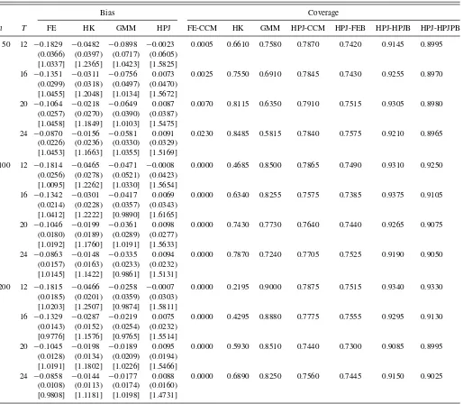
observationst =0 throughTfor estimation. This ensures that the results are not unduly influenced by the initial values of the process. In this case, we correctly fit panel AR(1) and there is no misspecification in the model. The results are collected in Table 1.
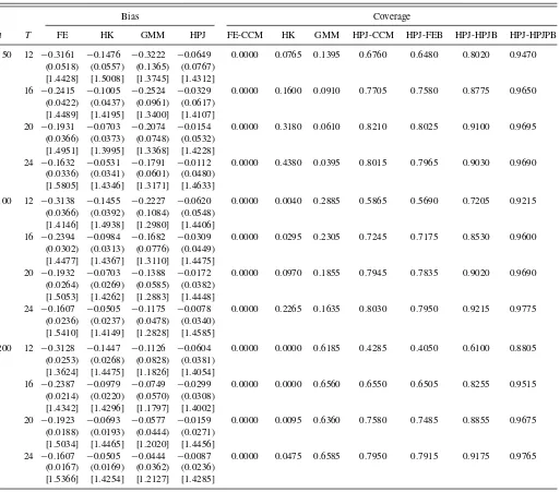
Table1: The FE estimate has large bias. The HK and GMM estimates are biased whenT andnare small, but the bias de-creases as T and n are large, respectively. The HPJ estimate is approximately unbiased. Regarding inference, the empirical coverage of FE-CCM is close to zero, likely due to the large bias in the FE estimate. HK is under coverage. GMM, as expected,
12However, Okui (2008) used a different set of assumptions and the sequential asymptotic scheme wheren→ ∞first and thenT → ∞, so his result is not directly transferred to our case. It is of interest to study the asymptotic properties of the GMM estimate under misspecification whennandTjointly go to infinity, which is left to future research.
has a good coverage property in this case, especially for largen. It is important to notice that the robust inference procedures, es-pecially HPJ–HPJB and HPJ–HPJPB, also have good coverage under no model misspecification.
In the next example, the true DGP follows a panel AR(2) model:
yit =ci+φ1yi,t−1+φ2yi,t−2+uit,
where uit ∼ iidt(10) andci∼ iidU(−0.5,0.5). Two cases
for the parametersφ1andφ2are considered:φ1=φ2=0.4 and
φ1=φ2 = −0.4. In generatingyitwe also setyi,−500=0.
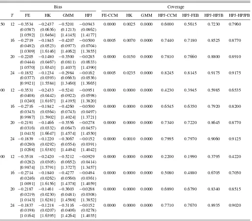
Despite that the true DGP is a panel AR(2) model, suppose that we incorrectly fit a panel AR(1) model and estimate the slope parameter. Whenφ1=φ2=0.4, the pseudo-true
param-eter isβ0=0.67, and whenφ1=φ2= −0.4,β0= −0.28. The
results for these two cases are presented in Tables 2 and 3, respectively.
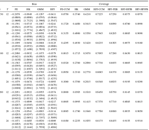
Table 2: The FE and GMM estimates are severely biased. The HK estimate is also biased as it is not designed for handling the case where misspecification is present. The HPJ estimate is able to reduce the bias substantially. The bias is small even for modestT, such asT =20 andT =24. Regarding the standard deviations, the HPJ estimate has slight variance inflation relative to the FE estimate in the finite sample (which is also observed in Dhaene and Jochmans (2009) in a different context of estimation of nonlinear panel data models such as panel probit models).
As for the empirical coverage, the FE-CCM, HK, and GMM options perform poorly because the FE, HK, and GMM es-timates are largely biased. The other options, namely, HPJ-CCM, HPJ-FEB, HPJ-HPJB, and HPJ-HPJPB, perform reason-ably well, but the HPJ-HPJPB option, as expected, seems to be the best. The coverage of HPJ-HPJPB is about 92% forn=100 andT =24, and close to the nominal 95%.
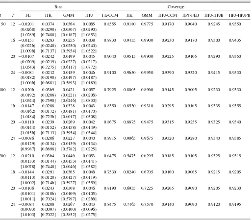
Table3: In this case, the incidental parameters bias is small and all the options perform relatively well. However, regarding
coverage, as n grows, the performance of the FE-CCM, HK,
and GMM options deteriorates since the ratio between the bias and the standard deviation becomes larger in each case. On the other hand, the other options, HPJ-CCM, HPJ-FEB, HPJ-HPJB and HPJ-HPJPB, perform well regardless of the combination of (n, T).
Table4: To extend the AR(2) example, we include exogenous regressors in the true DGP. In this case, the true DGP is as follows:
yit =ci+φ1yi,t−1+φ2yi,t−2+ρ1xi,t+ρ2xi,t−1+uit,
where uit∼ iid t(10), ci ∼ iid U(−0.5,0.5), and xit∼
iid N(0,1). We setyi,−500=0 and discard the first 500
ob-servations foryitandxit. Finally, the parametersφ1=φ2=0.4
andρ1=ρ2=0.5. In this case, we incorrectly fit a panel model
with regressors (yi,t−1, xi,t−1) and report estimates of the slope
parameter of the autoregressive term. This pseudo-true param-eter is β0=0.73. The results for this case are presented in
Table 4. The results inTable 4show evidence that the proposed methods are effective in finite sample. The bias of the HPJ es-timator is small, on the other hand the bias of other eses-timators are large. Regarding inference, given the bias in the FE, HK, and GMM, their respective coverage rates are poor. But the em-pirical coverage of HPJ-HPJB and HPJ-HPJPB are close to the nominal.
Table 1. Bias and empirical coverage for panel AR(1) model
Bias Coverage
n T FE HK GMM HPJ FE-CCM HK GMM HPJ-CCM HPJ-FEB HPJ-HPJB HPJ-HPJPB
50 12 −0.1829 −0.0482 −0.0898 −0.0023 0.0005 0.6610 0.7580 0.7870 0.7420 0.9145 0.8995 (0.0366) (0.0397) (0.0717) (0.0605)
[1.0337] [1.2365] [1.0423] [1.5825]
16 −0.1351 −0.0311 −0.0756 0.0073 0.0025 0.7550 0.6910 0.7845 0.7430 0.9255 0.8970 (0.0299) (0.0318) (0.0497) (0.0470)
[1.0455] [1.2048] [1.0134] [1.5672]
20 −0.1064 −0.0218 −0.0649 0.0087 0.0070 0.8115 0.6350 0.7910 0.7515 0.9305 0.8980 (0.0257) (0.0270) (0.0390) (0.0387)
[1.0458] [1.1849] [1.0103] [1.5475]
24 −0.0870 −0.0156 −0.0581 0.0091 0.0230 0.8485 0.5815 0.7840 0.7575 0.9210 0.8965 (0.0226) (0.0236) (0.0330) (0.0329)
[1.0453] [1.1663] [1.0355] [1.5169]
100 12 −0.1814 −0.0465 −0.0471 −0.0008 0.0000 0.4685 0.8500 0.7865 0.7490 0.9310 0.9250 (0.0256) (0.0278) (0.0521) (0.0423)
[1.0095] [1.2262] [1.0330] [1.5654]
16 −0.1342 −0.0301 −0.0417 0.0069 0.0000 0.6340 0.8255 0.7575 0.7385 0.9375 0.9105 (0.0214) (0.0228) (0.0357) (0.0343)
[1.0412] [1.2222] [0.9890] [1.6165]
20 −0.1046 −0.0199 −0.0361 0.0098 0.0000 0.7430 0.7730 0.7640 0.7440 0.9265 0.9075 (0.0180) (0.0189) (0.0289) (0.0277)
[1.0192] [1.1760] [1.0191] [1.5633]
24 −0.0863 −0.0148 −0.0335 0.0094 0.0000 0.7870 0.7240 0.7705 0.7525 0.9190 0.9050 (0.0157) (0.0163) (0.0233) (0.0232)
[1.0145] [1.1422] [0.9861] [1.5131]
200 12 −0.1815 −0.0466 −0.0258 −0.0007 0.0000 0.2195 0.9000 0.7875 0.7515 0.9340 0.9330 (0.0185) (0.0201) (0.0359) (0.0303)
[1.0203] [1.2507] [0.9874] [1.5811]
16 −0.1329 −0.0287 −0.0219 0.0075 0.0000 0.4295 0.8880 0.7775 0.7555 0.9295 0.9130 (0.0143) (0.0152) (0.0254) (0.0232)
[0.9776] [1.1576] [0.9765] [1.5514]
20 −0.1045 −0.0198 −0.0189 0.0095 0.0000 0.5930 0.8510 0.7440 0.7300 0.9085 0.8995 (0.0128) (0.0134) (0.0209) (0.0194)
[1.0191] [1.1802] [1.0226] [1.5466]
24 −0.0858 −0.0144 −0.0177 0.0088 0.0000 0.6890 0.8250 0.7560 0.7445 0.9150 0.9025 (0.0108) (0.0113) (0.0174) (0.0160)
[0.9808] [1.1181] [1.0198] [1.4731]
NOTES: Monte Carlo experiments based on 2000 repetitions. The standard deviations are inside parenthesis. Inside brackets are the ratio of the averages of the standard errors to the simulation of the standard deviations. The DGP isyit=ci+φyi,t−1+uit,with true parameterφ=0.8.
5.1.2 Random Coefficients AR Model. In the fourth exam-ple, the true DGP is
yit=ciyi,t−1+uit,
whereuit ∼ iidN(0,1),ci∼ iidU(0,0.9). This model appears
in Example 2 in Section2. As before, we incorrectly fit a panel AR(1) model and estimate the slope parameter. The value of the pseudo-true parameter isβ0=0.56. The simulation results for
this case are presented inTable 5.
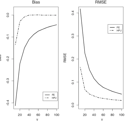
Table5: As in the previous cases, the FE estimate is largely biased and FE-CCM performs poorly due to the bias. Note that the decreasing speed of the standard deviation for the FE estimate asT grows is relatively slow, which would reflect the fact that the convergence rate of the FE estimate (without the bias part) under this DGP isn−1/2and not (nT)−1/2(the asymptotic
variance of the FE estimate consists of the part decreasing like
O(n−1) and also the part decreasing likeO
{(nT)−1
}, so even in this case, it is not surprising that the standard deviation of the FE estimate in the finite sample slowly decreases asT increases). The HPJ estimate is able to largely remove the bias, nevertheless there is slight variance inflation in the finite sample. In this example, the HK and GMM estimates are able to reduce the bias, to some extent, for large time series. However, the empirical coverage of the HK and GMM options are still poor. Lastly, among the inference procedures, HPJ-HPJPB works particularly well.
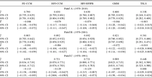
5.2 Real Data Analysis
In this section, we apply the procedures discussed in the previous sections to a model of unemployment dynamics at the U.S. state level. Bun and Carree (2005) and Baglan (2010)