07350015%2E2013%2E818005

(1)

Full Terms & Conditions of access and use can be found at

http://www.tandfonline.com/action/journalInformation?journalCode=ubes20

Download by: [Universitas Maritim Raja Ali Haji] Date: 11 January 2016, At: 22:18

Journal of Business & Economic Statistics

ISSN: 0735-0015 (Print) 1537-2707 (Online) Journal homepage: http://www.tandfonline.com/loi/ubes20

Factor-Augmented VARMA Models With

Macroeconomic Applications

Jean-Marie Dufour & Dalibor Stevanović

To cite this article: Jean-Marie Dufour & Dalibor Stevanović (2013) Factor-Augmented VARMA

Models With Macroeconomic Applications, Journal of Business & Economic Statistics, 31:4, 491-506, DOI: 10.1080/07350015.2013.818005

To link to this article: http://dx.doi.org/10.1080/07350015.2013.818005

Accepted author version posted online: 25 Aug 2013.

Submit your article to this journal

Article views: 275

(2)

Factor-Augmented VARMA Models

With Macroeconomic Applications

Jean-Marie DUFOUR

Department of Economics, McGill University, 855 Sherbrooke Street West, Leacock Building, Montreal, Quebec H3A 2T7, Canada (jean-marie.dufour@mcgill.ca)

Dalibor STEVANOVI´

C

D épartement des Sciences Économiques, Universit é du Qu ébec a Montr éal, 315 rue Ste-Catherine Est, Montr éal, Quebec H2X 3X2, Canada (dstevanovic.econ@gmail.com)

We study the relationship between vector autoregressive moving-average (VARMA) and factor representa-tions of a vector stochastic process. We observe that, in general, vector time series and factors cannot both follow finite-order VAR models. Instead, a VAR factor dynamics induces a VARMA process, while a VAR process entails VARMA factors. We propose to combine factor and VARMA modeling by using factor-augmented VARMA (FAVARMA) models. This approach is applied to forecasting key macroeconomic aggregates using large U.S. and Canadian monthly panels. The results show that FAVARMA models yield substantial improvements over standard factor models, including precise representations of the effect and transmission of monetary policy.

KEY WORDS: Factor analysis; Forecasting; Structural analysis; VARMA process.

1. INTRODUCTION

As information technology improves, the availability of eco-nomic and financial time series grows in terms of both time and cross-section size. However, a large amount of information can lead to a dimensionality problem when standard time series tools are used. Since most of these series are correlated, at least within some categories, their covariability and information con-tent can be approximated by a smaller number of variables. A popular way to address this issue is to use “large-dimensional approximate factor analysis,” an extension of classical factor analysis which allows for limited cross-section and time corre-lations among idiosyncratic components.

While factor models were introduced in macroeconomics and finance by Sargent and Sims (1977), Geweke (1977), and Chamberlain and Rothschild (1983), the literature on the large-factor models started with Forni et al. (2000) and Stock and Watson (2002a). Further theoretical advances were made, among others, by Bai and Ng (2002), Bai (2003), and Forni et al. (2004). These models can be used to forecast macroeconomic aggregates (Stock and Watson 2002b; Forni et al.2005; Banerjee, Marcellino, and Masten2006), structural macroeconomic analysis (Bernanke, Boivin, and Eliasz2005; Favero, Marcellino, and Neglia 2005), for nowcasting and economic monitoring (Giannone, Reichlin, and Small 2008; Aruoba, Diebold, and Scotti2009), to deal with weak instru-ments (Bai and Ng 2010; Kapetanios and Marcellino 2010), and the estimation of dynamic stochastic general equilibrium models (Boivin and Giannoni,2006).

Vector autoregressive moving-average (VARMA) models provide another way to obtain a parsimonious representation of a vector stochastic process. VARMA models are especially appropriate in forecasting, since they can represent the dynamic relations between time series while keeping the number of pa-rameters low; see L¨utkepohl (1987) and Boudjellaba, Dufour, and Roy (1992). Further, VARMA structures emerge as

reduced-form representations of structural models in macroeconomics. For instance, the linear solution of a standard dynamic stochas-tic general equilibrium model generally implies a VARMA rep-resentation on the observable endogenous variables (Ravenna

2006; Komunjer and Ng2011; Poskitt2011).

In this article, we study the relationship between VARMA and factor representations of a vector stochastic process, and we propose a new class of factor-augmented VARMA models. We start by observing that, in general, the multivariate time series and the associated factors do not typically follow finite-order VAR processes. When the factors are obtained as linear com-binations of the observable series, the dynamic process obeys a VARMA model, not a finite-order VAR as usually assumed in the literature. Further, if the latent factors follow a finite-order VAR process, this implies a VARMA representation for the observable series. Consequently, we propose to combine two techniques for representing in a parsimonious way the namic interactions between a huge number of time series: dy-namic factor reduction and VARMA modeling thus leading us to consider factor-augmented VARMA (FAVARMA) models. Besides parsimony, the class of VARMA models is closed un-der marginalization and linear transformations (in contrast with VAR processes). This represents an additional advantage if the number of factors is underestimated.

The importance of the factor process specification depends on the technique used to estimate the factor model and the research goal. In the two-step method developed by Stock and Watson (2002a), the factor process does not matter for the approximation of factors, but this might be an issue if we use a likelihood-based technique which relies on a completely specified process. Moreover, if predicting observable variables depend on factor

491

(3)

forecasting, a reliable and parsimonious approximation of the factor dynamic process is important. In Deistler et al. (2010), the authors studied identification of the generalized dynamic factor model where the common component has a singular rational spectral density. Under the assumption that transfer functions are tall and zeroless (i.e., the number of common shocks is less than the number of static factors), they argued that static factors have a finite-order AR singular representation which can be estimated by generalized Yule–Walker equations. Note that Yule–Walker equations are not unique for such systems, but Deistler, Filler, and Funovits (2011) proposed a particular canonical form for estimation purposes.

After showing that FAVARMA models yield a theoretically consistent specification, we study whether VARMA factors can help in forecasting time series. We compare the forecasting performance [in terms of Means Squared Error (MSE)] of four FAVARMA specifications, with standard AR(p),ARMA(p, q), and factor models where the factor dynamics is approximated by a finite-order VAR. An out-of-sample forecasting exercise is performed using a U.S. monthly panel from Boivin, Giannoni, and Stevanovi´c (2009a).

The results show that VARMA factors help in predicting sev-eral key macroeconomic aggregates, relative to standard factor models, and across different forecasting horizons. We find im-portant gains, up to a reduction of 42% in MSE, when forecast-ing the growth rates of industrial production, employment, and consumer price index inflation. In particular, the FAVARMA specifications generally outperform the VAR-factor forecast-ing models. We also report simulation results which show that VARMA factor modeling noticeably improves forecasting in finite samples.

Finally, we perform a structural factor analysis exercise. We estimate the effect of a monetary policy shock using the data and identification scheme of Bernanke, Boivin, and Eliasz (2005). We find that impulse responses from a parsimonious 6-factor FAVARMA(2,1) model give a precise and plausible picture of the effect and transmission of monetary policy in the United States. To get similar responses from a standard FAVAR model, the Akaike information criterion leads to a lag order of 14. So, we need to estimate 84 coefficients governing the factor dynamics in the FAVARMA framework, while the FAVAR model requires 510 VAR parameters.

In Section 2, we summarize some important results on lin-ear transformations of vector stochastic processes and present four identified VARMA forms. In Section3, we study the link between VARMA and factor representations. The FAVARMA model is proposed in Section4, and estimation is discussed in Section5. Monte Carlo simulations are discussed in Section6. The empirical forecasting exercise is presented in Section 7, and the structural analysis in Section8. Proofs and simulation results are reported in the Appendix.

2. FRAMEWORK

In this section, we summarize a number of important results on linear transformations of vector stochastic processes, and we present four identified VARMA forms that we will use in forecasting applications.

2.1 Linear Transformations of Vector Stochastic Processes

Exploring the features of transformed processes is important since data are often obtained by temporal and spatial aggre-gation, and/or transformed through linear filtering techniques, before they are used to estimate models and evaluate theories. In macroeconomics, researchers model dynamic interactions by specifying a multivariate stochastic process on a small num-ber of economic indicators. Hence, they work on marginalized processes, which can be seen as linear transformations of the original series. Finally, dimension-reduction methods, such as principal components, lead one to consider linear transforma-tions of the observed series. Early contributransforma-tions on these issues include Zellner and Palm (1974), Rose (1977), Wei (1978), Abraham (1982), and L¨utkepohl (1984).

The central result we shall use focuses on linear transforma-tions of an N-dimensional, stationary, strictly indeterministic stochastic process. SupposeXt satisfies the model

Xt =

∞

j=0

jεt−j =(L)εt, 0=IK, (2.1)

whereεt is a weak white-noise, withE(εt)=0,E(εtε′t)=ε,

det[ε]>0, E(XtX′t)=X, E(XtX′t+h)=ŴX(h), (L)=

∞

i=0iLi and det[(z)]=0 for|z|<1. (2.1) can be

inter-preted as the Wold representation of Xt, in which case εt =

Xt−PL[Xt|Xt−1, Xt−2, . . .] and PL[Xt|Xt−1, Xt−2, . . .]

is the best linear forecast ofXt based on its own past (i.e.,εt

is theinnovation processofXt). Consider the following linear

transformation ofXt

Ft =CXt, (2.2)

where C is aK×N matrix of rank K. Then,Ft is also

sta-tionary, indeterministic, and has zero mean, so it has an MA representation of the form

Ft=

∞

j=0

jvt−j =(L)vt, 0=IK, (2.3)

where vt is K-dimensional white-noise with E(vtvt′)=v.

These properties hold wheneverXt is a vector stochastic

pro-cess with an MA representation. If it is invertible, finite and infinite-order VAR processes are covered.

In practice, only a finite number of parameters can be esti-mated. Consider the MA(q) process

Xt =εt+M1εt−1+ · · · +Mqεt−q =M(L)εt (2.4)

with det[M(z)]=0 for |z|<1 and nonsingular white-noise noise covariance matrixε, and aK×N matrixCwith rank

K. Then, the transformed processFt =CXt has an invertible

MA(q∗) representation

Ft =vt+N1vt−1+ · · · +Nq∗vt−q∗ =N(L)vt (2.5)

with det[N(z)]=0 for |z|<1, wherevt is a K-dimensional

white-noise with nonsingular matrixv, each Ni is aK×K

coefficient matrix, andq∗ ≤q.

Some conditions in the previous results can be relaxed. The nonsingularity of the covariance matrixεand the full rank of

Care not necessary so there may be exact linear dependencies

(4)

among the components ofXt andFt; see L¨utkepohl (1984b). It

is also possible thatq∗< q.

It is well known that weak VARMA models are closed un-der linear transformations. LetXtbe anN-dimensional, stable,

invertible VARMA(p, q) process

(L)Xt =(L)εt, (2.6)

and let C be aK×N matrix of rankK < N. ThenFt=CXt

has a VARMA(p∗, q∗) representation with p∗≤(N−K+

1)p andq∗≤(N−K)p+q; see L¨utkepohl (2005, Corollary

11.1.2). A linear transformation of a finite-order VARMA pro-cess still has a finite-order VARMA representation, but with possibly higher autoregressive and moving-average orders.

When modeling economic time series, the most common specification is a finite-order VAR. Therefore, it is important to notice that this class of models is not closed with respect to linear transformations reducing the dimensions of the original process.

2.2 Identified VARMA Models

An identification problem arises since the VARMA represen-tation ofXt is not unique. There are several ways to identify

the process in Equation (2.6). In the following, we state four unique VARMA representations: the well-known final-equation form and three representations proposed in Dufour and Pelletier (2013).

Definition 2.1Final AR Equation Form (FAR). The VARMA representation in Equation (2.6) is said to be in final AR equation form if(L)=φ(L)IN, whereφ(L)=1−φ1L− · · · −φpLp

is a scalar polynomial withφp =0.

Definition 2.2 Final MA Equation Form (FMA). The VARMA representation in Equation (2.6) is said to be in fi-nal MA equation form if(L)=θ(L)IN, whereθ(L)=1−

θ1L− · · · −θqLq is a scalar polynomial withθq =0.

Definition 2.3 Diagonal MA Equation Form (DMA). The VARMA representation in Equation (2.6) is said to be in diagonal MA equation form if (L)=diag[θii(L)]=

IN−1L− · · · −qLq, where θii(L)=1−θii,1L− · · · −

θii,qiL

qi_{, θ}

ii,qi =0,andq =max1≤i≤N(qi).

Definition 2.4 Diagonal AR Equation Form (DAR). The VARMA representation in Equation (2.6) is said to be in diagonal AR equation form if (L)=diag[φii(L)]=

IN−1L− · · · −pLp, where φii(L)=1−φii,1L− · · · −

φii,piL

pi_{, φ}

ii,pi =0,andp=max1≤i≤N(pi).

The identification of these VARMA representations is discussed in Dufour and Pelletier (2013, Section 3). In particular, the identification of diagonal MA form is established under the simple assumption of no common root.

From standard results on the linear aggregation of VARMA processes (see, e.g., Zellner and Palm1974; Rose1977; Wei

1978; Abraham1982; L¨utkepohl1984), it is easy to see that an aggregated process such asFt also has an identified VARMA

representation in final AR or MA equation form. But this type of representation may not be attractive for several reasons. First, it is far from the usual VAR model, because it excludes lagged

values of other variables in each equation. Moreover, the AR coefficients are the same in all equations, which typically leads to a high-order AR polynomial. Second, the interaction between different variables is modeled through the MA part of the model, and may be difficult to assess in empirical and structural analy-sis.

The diagonal MA form is especially appealing. In contrast with the echelon form (Deistler and Hannan1981; Hannan and Deistler1988; L¨utkepohl1991, chap. 7), it is relatively simple and intuitive. In particular, there is no complex structure of zero off-diagonal elements in the AR and MA operators. For practitioners, this is quite appealing since adding lags of εit

to the ith equation is a simple natural extension of the VAR model. The MA operator has a simple diagonal form, so model nonlinearity is reduced and estimation becomes numerically simpler.

3. VARMA AND FACTOR REPRESENTATIONS

In this section, we study the link between VARMA and factor representations of a vector stochastic process Xt, and the

dy-namic process of the factors. In the theorems below, we suppose that Xt is an N-dimensional regular (strictly indeterministic)

discrete-time process inRN :X= {Xt :t ∈RN, t∈Z}with

Wold representation (2.1). In Theorem 3.1, we postulate a factor model forXtwhere factors follow a finite-order VAR process:

Xt =Ft+ut, (3.1)

where is anN×K matrix of factor loadings with rankK, andut is a (weak) white-noise process with covariance matrix

usuch that

E[Ftu′t]=0 for allt. (3.2)

We now show that finite-order VAR factors induce a finite-order VARMA process for the observable series. Proofs are supplied in the Appendix.

Theorem 3.1 Observable Process Induced by Finite-Order VAR Factors. SupposeXtsatisfies the Assumptions (3.1)–(3.2)

andFtfollows the VAR(p) process

Ft=(L)Ft−1+at (3.3)

such thatet =[ut...at]′is a (weak) white-noise process with

E[Ft−je′t]=0 forj ≥1, ∀t, (3.4)

(L)=1L− · · · −pLp, and the equation det[IK−

(z)]=0 has all its roots outside the unit circle. Then, for allt,E[Xt−je′t]=0 forj ≥1,andXt has the following

repre-sentations:

A(L)Xt =B(L)et, (3.5)

A(L)Xt =¯(L)εt, (3.6)

where A(L)=[I−(L)(′)−1′L],B(L)=[A(L)...], ¯

(L)=p+1

j=0¯jLj with ¯j = p+1

i=0 Aij−i, the matrices

j are the coefficients of the Wold representation (2.1),and

εtis the innovation process ofXt.

(5)

This result can be extended to the case where the factors have VARMA representations. It is not surprising that the induced process forXt is again a finite-order VARMA, though possibly

with a different MA order. This is summarized in the following theorem.

Theorem 3.2 Observable Process Induced by VARMA Factors. SupposeXt satisfies the Assumptions (3.1)–(3.2) and

Ftfollows the VARMA(p, q) process

Ft =(L)Ft−1+(L)at, (3.7)

where et =[ut...at]′ is a (weak) white-noise process which

satisfies the orthogonality condition (3.4), (L)=1L−

· · · −pLp, (L)=IK−1L− · · · −qLq, and the

equa-tion det[IK−(z)]=0 has all its roots outside the unit

circle. Then, Xt has representations of the form (3.5)

and (3.6),withB(L)=[A(L)...(L)],¯(L)=p∗

j=0¯jLj,

¯

j =

p∗

i=0Aij−i,andp∗=max(p+1, q).

Note that the usual invertibility assumption on the factor VARMA process (3.7) is not required. The next issue we con-sider concerns the factor representation of Xt. What are the

implications of the underlying structure ofXt on the

represen-tation of latent factors when the latter are calculated as linear transformations of Xt? This is summarized in the following

theorem.

Theorem 3.3 Dynamic Factor Models Associated with VARMA Processes. SupposeFt =CXt, whereCis aK×N

full-row rank matrix. Then, the following properties hold:

(i) ifXthas a VARMA(p, q) representation as in Equation

(2.6), then Ft has VARMA(p∗, q∗) representation with

p∗≤(N−K+1)pandq∗≤q+(N−K)p;

(ii) if Xt has a VAR(p) representation, then Ft has

VARMA(p∗, q∗) representation withp∗≤Npandq∗ ≤

(N−1)p;

(iii) ifXthas an MA representation as in Equation (2.4), then

Ft has an MA(q∗) representation withq ≤q∗.

From the Wold decomposition of common components, Deistler et al. (2010) argued that latent variables can have ARMA or state-space representations, but given the singular-ity and zero-free nature of transfer functions, they can also be modeled as finite-order singular AR processes. Theorem 3.3 does not assume the existence of a dynamic factor structure, so it holds for any linear aggregation ofXt.

Arguments in favor of using a FAVARMA specification can be summarized as follows:

(i) WheneverXt follows a VAR or a VARMA process, the

factors defined through a linear cross-sectional transfor-mation (such as principal components) follow a VARMA process. Moreover, a VAR or VARMA-factor structure on Xt entails a VARMA structure forXt.

(ii) VARMA representations are more parsimonious, so they easily lead to more efficient estimation and tests. As shown in Dufour and Pelletier (2013), the introduction of the MA operator allows for a reduction of the required AR order so we can get more precise estimates.

More-over, in terms of forecasting accuracy, VARMA models have theoretical advantages over the VAR representation (L¨utkepohl1987).

(iii) The use of VARMA factors can be viewed from two dif-ferent perspectives. First, if we use factor analysis as a dimension-reduction method, a VARMA specification is a natural process for factors (Theorem 3.3). Second, if factors are given a deep (“structural”) interpretation, the factor process has intrinsic interest, and a VARMA speci-fication on factors—rather than a finite-order VAR—is an interesting generalization motivated by usual arguments of theoretical coherence, parsimony, and marginalization. In particular, even ifFthas a finite-order VAR

representa-tion, subvectors ofFttypically follow a VARMA process.

4. FACTOR-AUGMENTED VARMA MODELS

We have shown that the observable VARMA process gener-ally induces a VARMA representation for factors, not a finite-order VAR. Following these results, we propose to consider factor-augmented VARMA (FAVARMA) models. Following the notation of Stock and Watson (2005), the dynamic factor model (DFM) where factors have a finite-order VARMA(pf, qf)

rep-resentation can be written as

Xit =λ˜i(L)ft+uit, (4.1)

uit =δi(L)ui,t−1+νit, (4.2)

ft =Ŵ(L)ft−1+(L)ηt,

i=1, . . . , N, t =1, . . . , T , (4.3)

where ft is a q×1 factor vector, ˜λi(L) is a 1×q

vec-tor of lag polynomials, ˜λi(L)=(˜λi1(L), . . . ,λ˜iq(L)),λ˜ij(L)=

pi, j

k=0λ˜i, j, kLk, δi(L) is apx,i-degree lag polynomial,Ŵ(L)=

Ŵ1L+ · · · +ŴpfL

pf_, ₍_L₎₌_I₋

1L− · · · −qfL

qf_{, and} νit is an N-dimensional white-noise uncorrelated with theq

-dimensional white-noise processηt. The exact DFM is obtained

if the following assumption is satisfied:

E(uituj s)=0, ∀i, j, t, s, i=j.

We obtain the approximate DFM by allowing for cross-section correlations among the idiosyncratic components as in Stock and Watson (2005). We assume the idiosyncratic errorsνit are

uncorrelated with the factorsftat all leads and lags.

On premultiplying both sides of Equation (4.1) by 1−δi(L),

we get the DFM with serially uncorrelated idiosyncratic errors:

Xit =λi(L)ft+δi(L)Xit−1+νit, (4.4)

where λi(L)=[1−δi(L)L]˜λi(L). Then, we can rewrite the

DFM in the following form:

Xt =λ(L)ft+D(L)Xt−1+νt, (4.5)

ft =Ŵ(L)ft−1+(L)ηt, (4.6)

(6)

where

To obtain the static version, we suppose thatλ(L) has degree p−1, and letFt =[ft′, f we obtain the static factor model which has been used to fore-cast time series (Stock and Watson2002b; Boivin and Ng2005; Stock and Watson2006), and study the impact of monetary pol-icy shocks in an FAVAR model (Bernanke, Boivin, and Eliasz

2005; Boivin, Giannoni, and Stevanovi´c2009a).

5. ESTIMATION

Several estimation methods have been proposed for factor models and VARMA processes (separately). One possibility is to estimate the system (4.7)–(4.9) simultaneously after making distributional assumptions on the error terms. This method is already computationally difficult when the factors have a simple VAR structure. Adding the MA part to the factor process makes this task even more difficult, for estimating VARMA models is typically not easy.

We use here the two-step Principal Component Analysis (PCA) estimation method; see Stock and Watson (2002a) and Bai and Ng (2008) for theoretical results concerning the PCA estimator. In the first step, ˆFtare computed asKprincipal

com-ponents ofXt. In the second step, we estimate the VARMA

representation (4.9) on ˆFt. The number of factors can be

esti-mated through different procedures proposed by Amengual and Watson (2007), Bai and Ng (2002), Bai and Ng (2007), Hallin and Liska (2007), and Onatski (2009a). In forecasting, we es-timate the number of factors using the Bayesian information criterion as in Stock and Watson (2002b), while the number of factors in the structural FAVARMA model is the same as in Bernanke, Boivin, and Eliasz (2005).

The standard estimation methods for VARMA models are maximum likelihood and nonlinear least squares. Unfortunately, these methods require nonlinear optimization, which may not be feasible when the number of parameters is large. Here, we use the GLS method proposed in Dufour and Pelletier (2013), which generalizes the regression-based estimation method introduced by Hannan and Rissanen (1982). Consider aK-dimensional zero

mean processYt generated by the VARMA(p, q) model:

A(L)Yt =B(L)Ut, (5.1)

whereA(L)=IK−A1L− · · · −ApLp,B(L)=IK−B1L−

· · · −BqLq, and Ut is a weak white-noise. Assume

det[A(z)]=0 for |z| ≤1 and det[B(z)]=0 for |z| ≤1 so the process Yt is stable and invertible. Set Ak=

[a′₁_•_,k, . . . , a_K′_•_,k]′, k=1, . . . , K, where aj•,k is thejth row

of Ak, and B(L)=diag[b11(L), . . . , bKK(L)], bjj(L)=1−

bjj,1L− · · · −bjj,qjL

qj_,_when_B₍_L_{) is in MA diagonal form.} Then, when the model is in diagonal MA form, we can write the parameters of the VARMA model as a vectorγ =[γ1, γ2]′

whereγ1contains the AR parameters andγ2the MA parameters,

as follows:

γ1 =[a1•,1, . . . , a1•,p, . . . , aK•,1, . . . , aK•,p], (5.2)

γ2 =[b11,1, . . . , b11,q1, . . . , bKK,1, . . . , bKK,qK]. (5.3) The estimation method involves three steps.

Step 1. Estimate a VAR(nT) model by least squares, where

nT < T /(2K), and compute the residuals:

t, that is, the corresponding estimate

of the covariance matrix ofUt, and apply GLS to the

multivariate regression

Step 3. Using the second step estimates, form new residuals

˜

(7)

with ˜Ut =0 fort ≤max(p, q),and define

The consistency and asymptotic normality of the above esti-mators were established by Dufour and Pelletier (2013). In the previous steps, the orders of the AR and MA operators are taken as known. In practice, they are usually estimated by statistical methods or suggested by theory. Dufour and Pelletier (2013) proposed an information criterion to be applied in the second step of the estimation procedure. For allpi ≤P andqi ≤Q,

compute

log[det( ˜U)]+dim(γ)

(logT)1+δ

T , δ >0. (5.10) Choose ˆpi and ˆqi as the set which minimizes the information

criteria (5.10). The properties of estimators ˆpi and ˆqi are given

in the article.

6. FORECASTING

In this section, we study whether the introduction of VARMA factors can improve forecasting. We consider a simplified ver-sion of the static model (4.7)–(4.9), whereFt is scalar:

Xit =λiFt+uit, (6.1)

uit =δiuit−1+νit, i, . . . , N, (6.2)

Ft =φFt−1+ηt−θ ηt−1. (6.3)

On replacingFt anduitin the observation Equation (6.1) with

the expressions in (6.2)–(6.3), we get the following forecast equation forXi,T+1based on the information available at time

T:

Xi,T+1|T =δiXiT +λi(φ−δi)FT −λiθ ηT.

Suppose λi =0, that is, there is indeed a factor structure

applicable toXit, andφ=δi, that is, the common and specific

components do not have the same dynamics. With the additional assumption thatFt follows an AR(1) process, Boivin and Ng

(2005) showed that taking into account the factor Ft allows

one to obtain better forecasts of Xit [in terms of the mean

squared error (MSE)]. We allow here for an MA component in the dynamic process ofFt, which provides a parsimonious way

of representing an infinite-order AR structure for the factor. Forecast performance depends on the way factors are esti-mated as well as the choice of forecasting model. Boivin and Ng (2005) considered static and dynamic factor estimation along with three types of forecast equations: (1)unrestricted, where Xi,T+h is predicted using XiT, FT, and their lags; (2) direct,

whereFT+his first predicted using its dynamic process, a

fore-cast is then used to predictXi,T+hwith the factor equation (6.3);

(3)nonparametric, where no parametric assumption is made on factor dynamics and its relationship with observables. The simu-lation and empirical results of Boivin and Ng (2005) showed that the unrestricted forecast equation with static factors generally yielded the best performance in terms of MSE.

6.1 Forecasting Models

A popular way to evaluate the predictive power of a model is to conduct an out-of-sample forecasting exercise. Here, we compare the FAVARMA approach with common factor-based methods. The forecast equations are divided in two categories. First, we consider methods where no explicit dynamic factor model is used, such as diffusion-index (DI) and diffusion au-toregressive (DI-AR) models (Stock and Watson2002b):

Xi,T+h|T =α(h)+

In this case, three variants are studied: (1) “unrestricted” (with m≥1 and p≥0); (2) “DI” (with m=1 and p=0); (3) “DI-AR” (with m=1). Second, we consider two-step meth-ods where common and specific components are first predicted from their estimated dynamic processes, and then combined to forecast the variables of interest using the estimated observa-tion equaobserva-tion. Moreover, we distinguish between sequential (or iterative) and direct methods to calculate forecasts (Marcellino, Stock, and Watson2006):

Xi,T+h|T =λ′iFT+h|T+ui,T+h|T,

where ui,T+h|T is obtained after fitting an AR(p) process

on uit, while the factor forecasts are obtained using

“se-quential” [FT+h|T =ˆT+h−1(L)FT+h−1|T] or “direct” methods

[FT+h|T =ˆ

(h)

T (L)FT].

In this exercise, the factors are defined as principal compo-nents ofXt. Thus, only the second type of forecast method is

affected by allowing for VARMA factors. We consider four iden-tified VARMA forms labeled: “Diag MA,” “Diag AR,” “Final MA,” and “Final AR.” The FAVARMA forecasting equations have the form:

Xi,T+h|T =λ′iFT+h|T+ui,T+h|T,

FT+h|T =ˆT+h−1(L)FT+h−1|T +ˆT+h−1(L)ηT+h−1|T.

Our benchmark forecasting model is an AR(p) model, as given by Stock and Watson (2002b) and Boivin and Ng (2005). However, given the postulated factor structure, a finite-order autoregressive model is only an approximation of the process of

(8)

Xit. From Theorem 3.1, the marginal process for each element of

Xttypically has an ARMA form. If the MA polynomial has roots

close to the noninvertibility region, a long autoregressive model may be needed to approximate the process. For this reason, we also consider ARMA models as benchmarks, to see how they fare with respect to AR and factor-based models.

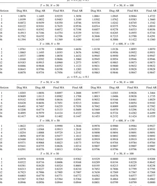
6.2 Monte Carlo Simulations

To assess the performance of our approach, we performed a Monte Carlo simulation comparing the forecasts of FAVARMA models (in four identified forms) with those of FAVAR mod-els. The data were simulated using a static factor model with MA(1) factors and idiosyncratic components similar to the ones considered by Boivin and Ng (2005) and Onatski (2009b):

Xit =λiFt+uit, Ft =ηt−Bηt−1,

uit =ρNui−1,t+ξit, ξit=ρTξi,t−1+ǫit,

ǫit ∼N(0,1), i =1, . . . , N, t =1, . . . , T ,

whereηt

iid

∼N(0,1),ρN ∈ {0.1,0.5,0.9}determines the

cross-sectional dependence,ρT ∈ {0.1,0.9}the time dependence, the

number of factors is 2,B=diag[0.5, 0.3],N = {50,100,130},

andT ∈ {50,100,600}. VARMA orders are estimated as given by Dufour and Pelletier (2013), the AR order for idiosyncratic component is 1, and the lag order in VAR approximation of factors dynamics is set to 6.

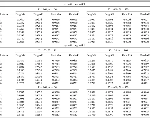
The results from this simulation exercise are presented in the Appendix (Table B.1). The numbers represent the MSE of four FAVARMA identified forms over the MSE of FAVAR direct forecasting models. When the number of time periods is small (T =50), FAVARMA models strongly outperform FAVAR models, especially at long horizons. The huge improve-ment at horizons 24 and 36 is due to the small sample size. When compared to the iterative FAVAR model (not reported), FAVARMA models still produce better forecasts in terms of MSE, but the improvement is smaller relative to the multi-step-ahead VAR-based forecasts. When the number of time periods increases (T =100, 600), the improvement of VARMA-based models is moderate, but the latter still yield better forecasts, especially at longer horizons. Another observation of interest is that FAVARMA models perform better when the factor structure is weak, that is, in cases where the cross-section size is relatively small (N =50 compared toN =100) and idiosyncratic com-ponents are correlated.

We performed additional simulation exercises (not re-ported), which also demonstrate a better performance of

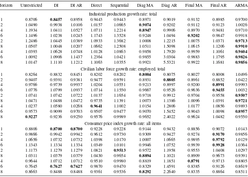
Table 1. RMSE relative to direct AR(p) forecasts

Horizon Unrestricted DI DI AR Direct Sequential Diag MA Diag AR Final MA Final AR ARMA

Industrial production growth rate: total

1 0.8706 0.8457 0.8958 0.9443 0.9443 0.8971 0.9019 0.9132 0.8985 0.9700 2 1.0490 0.9938 1.0106 1.0157 1.0665 0.9074 0.9202 0.9112 0.9123 1.0026 4 1.1934 1.0411 1.0527 1.0711 1.2214 0.8947 0.9906 0.8970 0.9481 0.9710 6 1.1496 1.0238 1.0245 1.1743 1.3528 0.9248 1.0494 0.9202 0.9847 0.9918 12 1.2486 1.0445 1.0389 1.0933 1.3682 1.0008 1.2215 1.0075 1.0371 0.9713

18 1.0507 1.0048 1.0207 1.0662 1.2508 1.0511 1.5098 1.0615 1.1206 0.9910

24 1.0393 1.0628 1.0748 1.0128 1.0863 0.9858 1.7920 0.9959 1.1061 0.9604

36 1.0092 1.0906 1.1437 1.2364 1.0421 0.9855 3.0304 0.9883 1.1795 0.9826

48 1.0147 1.1110 1.1212 1.1063 1.0355 0.9921 5.5321 0.9922 1.1681 0.9856

Civilian labor force growth rate: employed. total

1 0.8264 0.8832 0.8451 0.8202 0.8202 0.8004 0.8075 0.8027 0.8008 1.0496 2 0.9407 0.9391 0.9381 0.9477 0.9591 0.8931 0.8805 0.8961 0.8852 1.0422 4 0.9766 0.9739 0.9937 1.0204 1.0551 0.9213 0.8997 0.9200 0.8991 0.9993 6 1.0776 1.0799 1.0937 1.0714 1.1550 0.9667 0.9526 0.9636 0.9455 1.0032 12 1.0741 1.0742 1.0722 1.0137 1.1654 0.9718 0.9912 0.9704 0.9558 0.9507

18 1.0471 1.0488 1.0472 0.9735 1.1391 1.0073 1.1386 1.0096 1.0391 0.9721

24 1.0237 1.0580 1.0268 0.9641 1.1002 1.0154 1.2806 1.0177 1.0856 0.9893 36 0.9573 0.9099 0.9703 0.9507 0.9477 0.9070 1.5452 0.9043 1.0098 0.8957

48 0.9227 0.9236 0.9250 0.9576 0.9989 0.9652 2.4022 0.9624 1.0482 0.9550

Consumer price index growth rate: all items

1 0.8806 0.8700 0.8700 0.9228 0.9228 0.9144 0.9432 0.8856 0.9072 1.0143 2 0.9866 0.9942 0.9942 0.9612 0.9730 0.9309 0.9427 0.9274 0.9170 0.9856 4 1.0656 1.0732 1.0732 1.0398 1.0170 1.0007 1.0665 0.9895 0.9792 1.0129 6 1.1343 1.1334 1.1334 1.0349 1.0101 0.9946 1.0752 0.9939 0.9928 1.0364 12 1.1173 1.1279 1.1279 1.0821 0.9513 0.9572 1.1958 0.9553 1.0408 1.0297 18 1.0311 1.0379 1.0379 1.0430 0.9654 0.8894 1.1021 0.8909 0.9673 0.9391 24 0.9644 1.0712 1.0712 0.9510 0.9980 0.8819 1.1851 0.8791 0.9713 0.8805 36 0.7645 0.7627 0.7627 0.9870 0.9470 0.8329 1.4591 0.8385 0.9126 0.8619 48 0.8663 0.8488 0.8488 0.9361 0.9536 0.8292 2.2640 0.8335 0.8864 0.8511

NOTE: The numbers in bold character present the model producing the best forecasts in terms of MSE.

(9)

FAVARMA-based forecasts when the number of factors in-creases. The description and results are available in the online appendix version of Dufour and Stevanovi´c (2013a) and in the working article version of Dufour and Stevanovi´c (2013b).

7. APPLICATION: FORECASTING U.S. MACROECONOMIC AGGREGATES

In this section, we present an out-of-sample forecasting exer-cise using a balanced monthly panel from Boivin, Giannoni, and Stevanovi´c (2009a) that contained 128 monthly U.S. economic and financial indicators observed from 1959M01 to 2008M12. The series were initially transformed to induce stationarity.

The MSE results relative to benchmark AR(p) models are presented in Table 1. The out-of-sample evaluation period is 1988M01–2008M12. In the forecasting models “unrestricted,” “DI,” and “DI-AR,” the number of factors, the number of lags for both factors, andXitare estimated with BIC, and are allowed

to vary over the whole evaluation period. For the “unrestricted” model, the number of factors is 3,m=1, andp=0. In the case of “DI-AR” and “DI,” six factors are used, plus five lags ofXit

within the “DI-AR” representation.

In the FAVAR and FAVARMA models, the number of factors is set to 4. For all evaluation periods and forecasting horizons,

the estimated VARMA orders (AR and MA, respectively) are low: 1 and [1,1,1,1] for DMA form, [1,2,1,1] and 1 for DAR, 1 and 2 for FMA, and [2−4] and 1 for FAR form. The estimated VAR order is most of the time equal to 2, while the lag order of each idiosyncratic AR(p) process is between 1 and 3. In robustness analysis, the VAR order has been set to 4, 6, and 12, but the results did not change substantially. Both univariate ARMA orders are estimated to be 1, while the number of lags in the benchmark AR model fluctuates between 1 and 2.

The results inTable 1 show that VARMA factors improve the forecasts of key macroeconomic indicators across several horizons. For industrial production growth, the diffusion-index model exhibits the best performance at the one-month horizon, while the diagonal MA and final MA FAVARMA models out-perform the other methods for horizons of 2, 4, and 6 months. Fi-nally, the univariate ARMA models yield the smallest RMSE for the long-term forecasts. When forecasting employment growth, three FAVARMA forms outperform all other factor-based mod-els for short- and mid-term horizons. ARMA modmod-els still pro-duce the smallest RMSE for most of the long-term horizons.

For CPI inflation, the DI model provides the smallest MSE at horizon 1, while the final AR FAVARMA models do a better job at horizons 2, 4, and 6. Several VARMA-based models perform

Table 2. RMSE relative to ARMA(p, q) forecasts

Horizon Unrestricted DI DI AR Direct Sequential Diag MA Diag AR Final MA Final AR

1 0.8975 0.8719 0.9235 0.9735 0.9735 0.9248 0.9298 0.9414 0.9263

2 1.0463 0.9912 1.0080 1.0131 1.0637 0.9050 0.9178 0.9088 0.9099

4 1.2290 1.0722 1.0841 1.1031 1.2579 0.9214 1.0202 0.9238 0.9764

6 1.1591 1.0323 1.0330 1.1840 1.3640 0.9324 1.0581 0.9278 0.9928

12 1.2855 1.0754 1.0696 1.1256 1.4086 1.0304 1.2576 1.0373 1.0677

18 1.0602 1.0139 1.0300 1.0759 1.2622 1.0606 1.5235 1.0711 1.1308

24 1.0822 1.1066 1.1191 1.0546 1.1311 1.0264 1.8659 1.0370 1.1517

36 1.0271 1.1099 1.1640 1.2583 1.0606 1.0030 3.0841 1.0058 1.2004

48 1.0295 1.1272 1.1376 1.1225 1.0506 1.0066 5.6129 1.0067 1.1852

1 0.7873 0.8415 0.8052 0.7814 0.7814 0.7626 0.7693 0.7648 0.7630 2 0.9026 0.9011 0.9001 0.9093 0.9203 0.8569 0.8448 0.8598 0.8494 4 0.9773 0.9746 0.9944 1.0211 1.0558 0.9219 0.9003 0.9206 0.8997

6 1.0742 1.0765 1.0902 1.0680 1.1513 0.9636 0.9496 0.9605 0.9425

12 1.1298 1.1299 1.1278 1.0663 1.2258 1.0222 1.0426 1.0207 1.0054

18 1.0772 1.0789 1.0773 1.0014 1.1718 1.0362 1.1713 1.0386 1.0689

24 1.0348 1.0694 1.0379 0.9745 1.1121 1.0264 1.2945 1.0287 1.0973

36 1.0688 1.0159 1.0833 1.0614 1.0581 1.0126 1.7251 1.0096 1.1274

48 0.9662 0.9671 0.9686 1.0027 1.0460 1.0107 2.5154 1.0077 1.0976

1 0.8682 0.8577 0.8577 0.9098 0.9098 0.9015 0.9299 0.8731 0.8944

2 1.0010 1.0087 1.0087 0.9752 0.9872 0.9445 0.9565 0.9409 0.9304

4 1.0520 1.0595 1.0595 1.0266 1.0040 0.9880 1.0529 0.9769 0.9667

6 1.0945 1.0936 1.0936 0.9986 0.9746 0.9597 1.0374 0.9590 0.9579

12 1.0851 1.0954 1.0954 1.0509 0.9239 0.9296 1.1613 0.9277 1.0108

18 1.0980 1.1052 1.1052 1.1106 1.0280 0.9471 1.1736 0.9487 1.0300

24 1.0953 1.2166 1.2166 1.0801 1.1334 1.0016 1.3459 0.9984 1.1031

36 0.8870 0.8849 0.8849 1.1451 1.0987 0.9664 1.6929 0.9729 1.0588

48 1.0179 0.9973 0.9973 1.0999 1.1204 0.9743 2.6601 0.9793 1.0415

NOTE: The numbers in bold character present cases where the ARMA model outperforms the factor-based alternatives in terms of MSE.

(10)

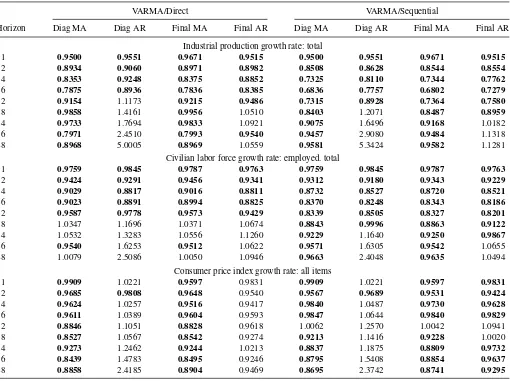
Table 3. MSE of FAVARMA relative to FAVAR forecasting models

VARMA/Direct VARMA/Sequential

Horizon Diag MA Diag AR Final MA Final AR Diag MA Diag AR Final MA Final AR

1 0.9500 0.9551 0.9671 0.9515 0.9500 0.9551 0.9671 0.9515

2 0.8934 0.9060 0.8971 0.8982 0.8508 0.8628 0.8544 0.8554

4 0.8353 0.9248 0.8375 0.8852 0.7325 0.8110 0.7344 0.7762

6 0.7875 0.8936 0.7836 0.8385 0.6836 0.7757 0.6802 0.7279

12 0.9154 1.1173 0.9215 0.9486 0.7315 0.8928 0.7364 0.7580

18 0.9858 1.4161 0.9956 1.0510 0.8403 1.2071 0.8487 0.8959

24 0.9733 1.7694 0.9833 1.0921 0.9075 1.6496 0.9168 1.0182

36 0.7971 2.4510 0.7993 0.9540 0.9457 2.9080 0.9484 1.1318

48 0.8968 5.0005 0.8969 1.0559 0.9581 5.3424 0.9582 1.1281

1 0.9759 0.9845 0.9787 0.9763 0.9759 0.9845 0.9787 0.9763

2 0.9424 0.9291 0.9456 0.9341 0.9312 0.9180 0.9343 0.9229

4 0.9029 0.8817 0.9016 0.8811 0.8732 0.8527 0.8720 0.8521

6 0.9023 0.8891 0.8994 0.8825 0.8370 0.8248 0.8343 0.8186

12 0.9587 0.9778 0.9573 0.9429 0.8339 0.8505 0.8327 0.8201

18 1.0347 1.1696 1.0371 1.0674 0.8843 0.9996 0.8863 0.9122

24 1.0532 1.3283 1.0556 1.1260 0.9229 1.1640 0.9250 0.9867

36 0.9540 1.6253 0.9512 1.0622 0.9571 1.6305 0.9542 1.0655

48 1.0079 2.5086 1.0050 1.0946 0.9663 2.4048 0.9635 1.0494

1 0.9909 1.0221 0.9597 0.9831 0.9909 1.0221 0.9597 0.9831

2 0.9685 0.9808 0.9648 0.9540 0.9567 0.9689 0.9531 0.9424

4 0.9624 1.0257 0.9516 0.9417 0.9840 1.0487 0.9730 0.9628

6 0.9611 1.0389 0.9604 0.9593 0.9847 1.0644 0.9840 0.9829

12 0.8846 1.1051 0.8828 0.9618 1.0062 1.2570 1.0042 1.0941

18 0.8527 1.0567 0.8542 0.9274 0.9213 1.1416 0.9228 1.0020

24 0.9273 1.2462 0.9244 1.0213 0.8837 1.1875 0.8809 0.9732

36 0.8439 1.4783 0.8495 0.9246 0.8795 1.5408 0.8854 0.9637

48 0.8858 2.4185 0.8904 0.9469 0.8695 2.3742 0.8741 0.9295

NOTE: The numbers in bold character present cases where the FAVARMA model performs better than the FAVAR.

the best for longer horizons (18, 24, and 48 months), while sequential and DI approaches dominate in forecasting 12 and 36 months ahead.

From Theorem 3.1, it is easy to see that each component of Xtfollows a univariate ARMA process. The forecasts based on

factor and univariate ARMA models are not in general equiva-lent, because different information sets are used. Even though multivariate models (such as factor models) use more variables, univariate ARMA models tend to be more parsimonious in prac-tice, which may reduce estimation uncertainty. So, these two modeling strategies can produce quite different forecasts. In

Table 2, we present MSE of all factor model predictions relative to ARMA forecasts. Boldface numbers highlight cases where the ARMA model outperforms the factor-based alternatives in terms of MSE.

For industrial production, ARMA specifications do better than all diffusion-index and FAVAR models (except at the one-month horizon). For employment, the conclusion is quite similar relative to FAVARMA, while diffusion-index models perform better than ARMA at horizons 1, 2, 4, and 48. Finally, in the case of CPI inflation, the ARMA model seems to be a better choice for most of the horizons relative to diffusion-index and

FAVAR alternatives. On the other hand, FAVARMA models do much better, for example, the final MA form beats the ARMA models at all horizons.

Based on these results, ARMA models appears to be a very good alternative to standard factor-based models at long hori-zons. This is not surprising since ARMA models are very par-simonious. However, FAVARMA models outperform ARMA models in most cases.

It is also of interest to see more directly how FAVARMA forecasts compare to those from FAVAR models. InTable 3, we present MSE of FAVARMA forecasting models relative to Di-rect and Sequential FAVAR specifications. The numbers in bold character present cases where the FAVARMA model performs better than the FAVAR.

Most numbers inTable 3are boldfaced, that is, FAVARMA models outperform standard FAVAR specifications at most hori-zons. This is especially the case for industrial production, where both MA VARMA forms produce smaller MSE at all horizons. At best, the FAVARMA model improves the forecasting accu-racy by 32% at horizon 12. In the case of Civilian labor force, VARMA factors do improve the predicting power, but the Di-rect FAVAR model performs better for longer horizons. Finally,

(11)

Figure 1. FAVARMA-DMA impulse responses to monetary policy shock. The online version of this figure is in color.

(12)

Figure 2. Comparison between FAVAR and FAVARMA impulse responses to a monetary policy shock. The online version of this figure is in color.

(13)

both diagonal and final MA FAVARMA specifications provide smaller MSEs over all horizons in predicting CPI inflation. The improvement increases with the forecast horizons, and reaches a maximum of 15%.

We performed a similar exercise with a Canadian dataset from Boivin, Giannoni, and Stevanović (2009b). We found that VARMA factors help in predicting several key Canadian macroeconomic aggregates, relative to standard factor models, and at many forecasting horizons. The description and results are available in the online appendix of Dufour and Stevanović (2013a) and in the working article version of Dufour and Stevanović (2013b).

8. APPLICATION: EFFECTS OF MONETARY POLICY SHOCKS

In the recent empirical macroeconomic literature, structural factor analysis has become popular: using hundreds of observ-able economic indicators appears to overcome several difficul-ties associated with standard structural VAR modeling. In par-ticular, bringing more information, while keeping the model parsimonious, may provide corrections for omitted and mea-surement errors; see Bernanke, Boivin, and Eliasz (2005) and Forni et al. (2009).

We reconsider the empirical study of Bernanke, Boivin, and Eliasz (2005) with the same data, the same method to extract factors (principal components), and the same observed factor (Federal Funds Rate). So, we set D(L)=0 and G=I in Equations (4.8)–(4.9). The difference is that we estimate VARMA dynamics on static factors instead of imposing a finite-order VAR representation. The monetary policy shock is identi-fied from the Cholesky decomposition of the residual covariance matrix in Equation (4.9), where the observed factor is ordered last. We consider all four identified VARMA forms, but retain only the diagonal MA representation. The number of latent fac-tors is set to five, and we estimate a VARMA (2.1) model [these orders were estimated using the information criterion in Dufour and Pelletier (2013)].

InFigure 1, we present FAVARMA(2,1)-based impulse re-sponses, with 90% confidence intervals (computed from 5000 bootstrap replications). A contractionary monetary policy shock generates a significant and very persistent economic downturn. The confidence intervals are more informative than those from FAVAR models. We conclude that impulse responses from a parsimonious 6-factor FAVARMA(2, 1) model provide a precise and plausible picture of the effect and transmission of monetary policy in the United States.

In Figure 2, we compare the impulse responses to a mone-tary policy shock estimated from FAVAR and FAVARMA-DMA models. The FAVAR impulse coefficients were computed for several VAR orders. To get similar responses from a standard FAVAR model, the Akaike information criterion leads to a lag order of 14. So, we need to estimate 84 coefficients governing the factors dynamics in the FAVARMA framework, while the FAVAR model requires 510 VAR parameters.

The approximation of the true factor process could be im-portant when choosing the parametric bootstrap procedure to obtain statistical inference on objects of interest. The confi-dence intervals are produced as follows [see Yamamoto (2011) for theoretical justification of this bootstrap procedure].

Step 1. Shuffle the time periods, with replacement, of the residuals in Equation (4.9) to get the bootstrap sam-ple ˜ηt.Then, resample static factors using estimated

VARMA coefficients:

˜

Ft =ˆ(L) ˜Ft−1+ˆη˜t.

Step 2. Shuffle the time periods, with replacement, of the residuals in Equation (4.7) to get the bootstrap sample

˜

ut. Then, resample the observable series using ˜Ftand

the estimated loadings:

˜

Xt =ˆF˜t+u˜t.

Step 3. Estimate FAVARMA model on ˜Xt, identify structural

shocks, and produce impulse responses.

9. CONCLUSION

In this article, we have studied the relationship between VARMA and factor representations of a vector stochastic pro-cess and proposed the FAVARMA model. We started by ob-serving that multivariate time series and their associated factors cannot in general both follow a finite-order VAR process. When the factors are obtained as linear combinations of observable series, the dynamic process of the latter has a VARMA struc-ture, not a finite-order VAR form. In addition, even if the factors follow a finite-order VAR process, this implies a VARMA rep-resentation for the observable series. As a result, we proposed the FAVARMA framework, which combines two parsimonious methods to represent the dynamic interactions between a large number of time series: factor analysis and VARMA modeling.

To illustrate the performance of the proposed approach, we performed Monte Carlo simulations and found that VARMA modeling is quite helpful, especially in small-sample cases— where the best improvement occurred at long horizons—but also in cases where the sample size is comparable to the one in our empirical data.

We applied our approach in an out-of-sample forecasting ex-ercise based on a large U.S. monthly panel. The results show that VARMA factors help predict several key macroeconomic aggregates relative to standard factor models. In particular, FAVARMA models generally outperform FAVAR forecasting models, especially if we use MA VARMA-factor specifications. Finally, we estimated the effect of monetary policy using the data and the identification scheme of Bernanke, Boivin, and Eliasz (2005). We found that impulse responses from a parsi-monious 6-factor FAVARMA (2.1) model yield a precise and plausible picture of the effect and the transmission of monetary policy in the United States. To get similar responses from a standard FAVAR model, the Akaike information criterion leads to a lag order of 14. So, we need to estimate 84 coefficients governing the factor dynamics in the FAVARMA framework, while the FAVAR model requires 510 parameters.

APPENDIX

A. PROOFS

Proof of Theorem 3.1. Sincehas full rank, we can multiply Equation (3.1) by (′)−1′to get

Ft−1=(′)−1′Xt−1−(′)−1′ut−1. (A.1)

(14)

Table B.1. Comparison between FAVARMA and FAVAR forecasts: Monte Carlo simulations

ρT =0.9, ρN =0.5

T =50, N=50 T =50,N=100

1 1.0078 1.1405 0.9235 1.3858 1.0061 1.0945 0.9084 1.4722

2 1.0199 1.0852 0.9483 1.3189 1.0302 1.0762 0.9383 1.3660

4 0.8872 0.9459 0.8350 1.0746 0.9338 1.0242 0.8745 1.1542

6 0.8122 0.9181 0.7635 0.9536 0.8514 0.9375 0.7954 1.0010

12 0.6311 0.8392 0.6072 0.7198 0.6857 0.9278 0.6533 0.8036

18 0.4913 0.7186 0.4754 0.5339 0.5181 0.8285 0.4955 0.5744

24 0.3762 0.6192 0.3706 0.4237 0.3846 0.7215 0.3788 0.4291

36 0.1394 0.2429 0.1369 0.1480 0.1445 0.3006 0.1422 0.1560

T =100,N=50 T =600,N =130

1 1.0761 1.1170 1.0004 1.6656 1.0130 1.0126 1.0093 1.0070

2 1.0865 1.1495 1.0193 1.5676 0.9962 0.9956 0.9952 0.9951

4 1.0537 1.0890 1.0038 1.4432 0.9945 0.9950 0.9947 0.9947

6 1.0168 1.0392 0.9686 1.3060 0.9945 0.9954 0.9946 0.9946

12 0.9183 0.9915 0.8960 1.2573 0.9871 0.9883 0.9873 0.9873

18 0.8886 0.9848 0.8552 1.1123 0.9831 0.9880 0.9832 0.9832

24 0.8643 0.9706 0.8198 1.1203 0.9831 0.9830 0.9828 0.9828

36 0.8078 0.9754 0.7956 1.0742 0.9863 0.9846 0.9847 0.9847

ρT =0.9, ρN =0.1

T =50,N=50 T =50,N=100

1 1.0203 1.0656 0.8897 1.2688 0.9977 1.0303 0.9026 1.3464

2 0.9689 1.0113 0.8982 1.1708 1.0013 1.0406 0.9038 1.1735

4 0.9142 0.9508 0.8616 1.0391 0.9032 0.9166 0.8461 1.0029

6 0.8420 0.8656 0.7851 0.9213 0.8841 0.8798 0.8054 0.9182

12 0.6401 0.7487 0.6235 0.7038 0.7042 0.8089 0.6850 0.7582

18 0.5208 0.6774 0.5133 0.5609 0.5469 0.6970 0.5296 0.5742

24 0.4095 0.5979 0.4124 0.4322 0.4380 0.5724 0.4282 0.4499

36 0.1417 0.2169 0.1402 0.1447 0.1453 0.2152 0.1424 0.1535

T =100,N=50 T =600,N =130

1 1.0622 1.0751 0.9990 1.3846 0.9978 0.9980 0.9984 0.9927

2 1.0578 1.0368 0.9913 1.2818 0.9935 0.9951 0.9935 0.9933

4 1.0254 1.0088 0.9729 1.2141 0.9890 0.9894 0.9891 0.9891

6 1.0058 0.9720 0.9477 1.1812 0.9892 0.9892 0.9892 0.9892

12 0.9480 0.9163 0.8819 1.0303 0.9919 0.9918 0.9919 0.9919

18 0.9371 0.9068 0.8823 1.0173 0.9784 0.9784 0.9784 0.9784

24 0.9441 0.8755 0.8626 1.0214 0.9807 0.9807 0.9807 0.9807

36 0.8591 0.8376 0.8013 0.9264 0.9796 0.9796 0.9796 0.9796

T =50,N=50 T =50,N=100

1 0.8978 0.9108 0.8924 0.9362 0.9329 0.8880 0.8585 0.9208

2 0.8522 0.8716 0.8606 0.9168 0.8289 0.8194 0.8228 0.8642

4 0.8381 0.8420 0.8524 0.8601 0.8195 0.8213 0.8187 0.8238

6 0.8213 0.8227 0.8225 0.8210 0.7852 0.7806 0.7799 0.7795

12 0.7923 0.7906 0.7905 0.7907 0.7630 0.7569 0.7567 0.7568

18 0.6803 0.6770 0.6771 0.6772 0.6582 0.6576 0.6577 0.6577

24 0.5367 0.5363 0.5364 0.5364 0.4865 0.4864 0.4863 0.4862

36 0.0946 0.0956 0.0944 0.0944 0.0801 0.0799 0.0799 0.0800

(Continued on next page)

(15)

Table B.1. Comparison between FAVARMA and FAVAR forecasts: Monte Carlo simulations(Continued)

ρT =0.1, ρN=0.9

T =100,N =50 T =600,N=130

1 0.9680 0.9676 0.9560 0.9515 0.9931 0.9995 0.9926 0.9921

2 0.9332 0.9304 0.9306 0.9310 0.9881 0.9929 0.9882 0.9878

4 0.9338 0.9261 0.9257 0.9257 0.9882 0.9895 0.9893 0.9894

6 0.9467 0.9350 0.9351 0.9351 0.9831 0.9831 0.9830 0.9830

12 0.9358 0.9359 0.9359 0.9359 0.9825 0.9825 0.9825 0.9825

18 0.9297 0.9298 0.9297 0.9297 0.9874 0.9873 0.9873 0.9873

24 0.9140 0.9142 0.9143 0.9143 0.9887 0.9886 0.9886 0.9886

36 0.9044 0.9047 0.9043 0.9043 0.9929 0.9930 0.9930 0.9930

ρT =0.1, ρN=0.1

T =50,N=50 T =50,N =100

1 0.9439 0.8761 0.7969 0.9618 0.9289 0.8919 0.8155 0.9675

2 0.8029 0.7863 0.7764 0.8459 0.7888 0.7900 0.7736 0.8569

4 0.7894 0.7542 0.7533 0.7742 0.7513 0.7533 0.7525 0.7687

6 0.7580 0.7420 0.7409 0.7438 0.7477 0.7488 0.7446 0.7458

12 0.6773 0.6751 0.6751 0.6754 0.6575 0.6604 0.6560 0.6613

18 0.5757 0.5700 0.5701 0.5761 0.5741 0.5753 0.5704 0.5728

24 0.4106 0.4074 0.4073 0.4084 0.4329 0.4303 0.4304 0.4317

36 0.0726 0.0721 0.0721 0.0721 0.0719 0.0722 0.0721 0.0721

T =100,N =50 T =600,N=130

1 0.9702 0.9672 0.9290 0.9316 0.9838 0.9874 0.9868 0.9840

2 0.8998 0.9053 0.8985 0.8993 0.9816 0.9904 0.9811 0.9811

4 0.9095 0.9003 0.9000 0.8997 0.9891 0.9894 0.9891 0.9891

6 0.8806 0.8771 0.8767 0.8767 0.9821 0.9822 0.9821 0.9821

12 0.8855 0.8841 0.8839 0.8839 0.9778 0.9778 0.9778 0.9778

18 0.8725 0.8704 0.8702 0.8702 0.9852 0.9852 0.9852 0.9852

24 0.8711 0.8707 0.8709 0.8709 0.9815 0.9815 0.9815 0.9815

36 0.8183 0.8185 0.8183 0.8183 0.9790 0.9790 0.9790 0.9790

If we now substituteFt−1in Equation (3.3), we see that

Ft=(L)(′)−1′Xt−1−(L)(′)−1′ut−1+at,

hence, on substituting the latter expression forFt in Equation

(3.1), and definingA1(L)=(L)(′)−1′,

Xt =Ft+ut=A1(L)Xt−1+ut−A1(L)ut−1+at

=A1(L)Xt−1+A(L)ut+at=A1(L)Xt−1+B(L)et,

where A(L)=I−A1(L)L andet =[ut...at]′. This yields the

representation (3.5).

We will now show thatXtcan be written as a VARMA process

where the noise is the innovation process of Xt.Since Xt is

regular strictly indeterministic weakly stationary process, it has a moving-average representation of the form (2.1), whereεt =

Xt−PL[Xt|Xt−1, Xt−2, . . .] and PL[Xt|Xt−1, Xt−2, . . .]

is the best linear forecast of Xt based on its own past, ε=

E[εtε′t] and det[ε]>0.Using the Assumptions (3.2) and (3.4),

it is easy to see that

E[Xt−ju′t]=E[Xt−jat′]=E[utε′t−j]

=E[atεt′−j]=0 forj ≥1. (A.2)

Then,

A(L)Xt =A(L)(L)εt=¯(L)εt=

∞

j=0

¯

jεt−j, (A.3)

where ¯j = p+1

i=0 Aij−i ands=0 fors <0, s=j−i.

Let us now multiply A(L)Xt by ε′t−k and take the expected

value: using Equations (A.3) and (3.5), we get

E[A(L)Xtε′t−k]=

∞

j=0

¯

jE[εt−jεt′−k]=Bjε (A.4)

=E[(A(L)ut+at)εt′−k]=0 fork > p+1.

(A.5)

(16)

Hence, ¯j =0 for k > p+1, so that Xt has the following

Proof of Theorem 3.2. To obtain the representations of Xt,

we follow the same steps as in the previous proof except that we substitute Equation (A.1) forFt−1in Equation (3.7), which

yields

Xt =(L)(′)−1′Xt−1+ut−(L)(′)−1′ut−1

+(L)at.

DefiningA(L) andet as above, withB(L)=[A(L)...(L)],

gives the representation as in Equation (3.5). Then, we remark that Equation (A.5) becomes

E[(A(L)ut+(L)at)εt′−k]=0 fork >max(p+1, q),

(A.7)

soXthas a VARMA (p+1,max(p+1, q)).

Proof of Theorem 3.3. Ft=CXt, whereCis aK×N

full-row rank matrix. Properties (i) and (ii) are easily proved using L¨utkepohl (2005, Corollaries 11.1.1 and 11.1.2). For (iii), ifXt

has an MA representation as in Equation (2.1) or Equation (2.4), the result is obtained using L¨utkepohl (1987, Propositions 4.1

and 4.2).

B. SIMULATION RESULTS: FAVARMA AND FAVAR FORECASTS

Table B.1contains the results of the Monte Carlo simulation exercise presented in Section6.2. The numbers represent the MSE of four FAVARMA identified forms over the MSE of FAVAR direct forecasting models.

[Received April 2012. Revised June 2013.]

REFERENCES

Abraham, B. (1982), “Temporal Aggregation and Time Series,”International Statistical Review, 50, 285–291. [492,493]

Amengual, D., and Watson, M. (2007), “Consistent Estimation of the Number of Dynamic Factors in Large N and T Panel,”Journal of Business and Economic Statistics, 25, 91–96. [495]

Aruoba, S., Diebold, F., and Scotti, C. (2009), “Real-Time Measurement of Business Conditions,”Journal of Business and Economic Statistics, 27, 417–427. [491]

Bai, J. (2003), “Inferential Theory for Factor Models of Large Dimensions,”

Econometrica, 71, 135–172. [491]

Bai, J., and Ng, S. (2002), “Determining the Number of Factors in Approximate Factor Models,”Econometrica, 70, 191–221. [491,495]

——— (2007), “Determining the Number of Primitive Shocks,”Journal of Business and Economic Statistics, 25, 52–60. [495]

——— (2008), “Large Dimensional Factor Analysis,”Foundations and Trends in Econometrics, 3, 89–163. [495]

——— (2010), “Instrumental Variable Estimation in a Data-Rich Environment,”

Econometric Theory, 26, 1577–1606. [491]

Banerjee, A., Marcellino, M., and Masten, I. (2008), “Forecasting Macroeco-nomic Variables Using Diffusion Indexes in Short Samples With Structural

Change,” inForecasting in the Presence of Structural Breaks and Model Un-certainty, eds. D. Rapach and M. Wohar, UK: Emerald Group Publishing, Ltd. [491]

Bernanke, B., Boivin, J., and Eliasz, P. (2005), “Measuring the Effects of Mon-etary Policy: A Factor-Augmented Vector Autoregressive (FAVAR) Ap-proach,”Quarterly Journal of Economics, 120, 387–422. [491,492,495,502] Boivin, J., and Giannoni, M. (2006), “DSGE Models in a Data-Rich Environ-ment,” Technical Report, Columbia Business School, Columbia University. [491]

Boivin, J., Giannoni, M., and Stevanovi´c, D. (2009a), “Dynamic Effects of Credit Shocks in a Data-Rich Environment,” Technical Report, Columbia Business School, Columbia University. [492,495,498]

——— (2009b), “Monetary Transmission in a Small Open Economy: More Data, Fewer Puzzles,” Technical Report, Columbia Business School, Columbia University. [502]

Boivin, J., and Ng, S. (2005), “Understanding and Comparing Factor-Based Forecasts,”International Journal of Central Banking, 1, 117–151. [495,496,497]

Boudjellaba, H., Dufour, J.-M., and Roy, R. (1992), “Testing Causality Between Two Vectors in Multivariate ARMA Models,” Journal of the American Statistical Association, 87, 1082–1090. [491]

Chamberlain, G., and Rothschild, M. (1983), “Arbitrage, Factor Structure and Mean-Variance Analysis in Large Asset Markets,”Econometrica, 51, 1281– 1304. [491]

Deistler, M., Anderson, B., Filler, A., Zinner, C., and Chen, W. (2010), “Gener-alized Linear Dynamic Factor Models—An Approach via Singular Autore-gressions,”European Journal of Control, 16, 211–224. [492,494] Deistler, M., Filler, A., and Funovits, B. (2011), “AR Systems and AR Processes:

The Singular Case,”Communications in Information and Systems, 11, 225– 236. [492]

Deistler, M., and Hannan, E. J. (1981), “Some Properties of the Parameterization of ARMA Systems With Unknown Order,”Journal of Multivariate Analysis, 11, 474–484. [493]

Dufour, J.-M., and Pelletier, D. (2013), “Practical Methods for Modeling Weak VARMA Processes: Identification, Estimation and Specification With a Macroeconomic Application,” Technical Report, Department of Eco-nomics, McGill University, CIREQ and CIRANO, Montr´eal, Canada. [493,494,495,496,497,502]

Dufour, J.-M., and Stevanovi´c, D. (2013a), “Factor-Augmented VARMA Mod-els With Macroeconomic Applications: Online Appendix,” Technical Re-port, Department of Economics, McGill University, Montr´eal, Canada. [498,502]

——— (2013b), “Factor-Augmented VARMA Models With Macroeconomic Applications,” Technical Report, Department of Economics, McGill Uni-versity, Montr´eal, Canada. [498,502]

Favero, C., Marcellino, M., and Neglia, F. (2005), “Principal Components at Work: The Empirical Analysis of Monetary Policy With Large Datasets,”

Journal of Applied Econometrics, 20, 603–620. [491]

Forni, M., Giannone, D., Lippi, M., and Reichlin, L. (2009), “Opening the Black Box: Identifying Shocks and Propagation Mechanisms in VAR and Factor Models,”Econometric Theory, 25, 1319–1347. [502]

Forni, M., Hallin, M., Lippi, M., and Reichlin, L. (2000), “The Generalized Factor Model: Identification and Estimation,”The Review of Economics and Statistics, 82, 540–554. [491]

——— (2004), “The Generalized Factor Model: Consistency and Rates,” Jour-nal of Econometrics, 119, 231–255. [491]

——— (2005), “The Generalized Dynamic Factor Model: One-Sided Estima-tion and Forecasting,”Journal of the American Statistical Association, 100, 830–839. [491]

Geweke, J. (1977), “The Dynamic Factor Analysis of Economic Time Series,” in Latent Variables in Socio Economic Models, eds. D. Aigner and A. Goldberger, Vol. 77, Amsterdam: North Holland, pp. 304–313. [491] Giannone, D., Reichlin, L., and Small, D. (2008), “Nowcasting: The

Real-Time Informational Content of Macroeconomic Data,”Journal of Monetary Economics, 55, 665–676. [491]

Hallin, M., and Liska, R. (2007), “Determining the Number of Factors in the General Dynamic Factor Model,”Journal of the American Statistical Asso-ciation, 102, 603–617. [495]

Hannan, E. J., and Deistler, M. (1988),The Statistical Theory of Linear Systems, New York: Wiley. [493]

Hannan, E. J., and Rissanen, J. (1982), “Recursive Estimation of Mixed Autoregressive-Moving-Average Order,”Biometrika, 69, 81–94. Errata 70 (1983), 303. [495]

Kapetanios, G., and Marcellino, M. (2010), “Factor-GMM Estimation With Large Sets of Possibly Weak Instruments,”Computational Statistics and Data Analysis, 54, 2655–2675. [491]

Komunjer, I., and Ng, S. (2011), “Dynamic Identification of Dynamic Stochastic General Equilibrium Models,” Econometrica, 79, 1995–2032. [491]

(17)

L¨utkepohl, H. (1984), “Forecasting Contemporaneously Aggregated Vector ARMA Processes,”Journal of Business and Economic Statistics, 2, 201– 214. [492,493]

——— (1984b), “Linear Transformations of Vector ARMA Processes,”Journal of Econometrics, 26, 283–293. [493]

——— (1987), Forecasting Aggregated Vector ARMA Processes, Berlin: Springer-Verlag. [491,494,505]

——— (1991),Introduction to Multiple Time Series Analysis, Berlin: Springer-Verlag. [493]

——— (2005),New Introduction to Multiple Time Series Analysis, Berlin, Germany: Springer-Verlag. [493,505]

Marcellino, M., Stock, J. H., and Watson, M. W. (2006), “A Comparison of Direct and Iterated Multistep ar Methods for Forecasting Macroeconomic Time Series,”Journal of Econometrics, 135, 499–526. [496]

Onatski, A. (2009a), “A Formal Statistical Test for the Number of Fac-tors in the Approximate Factor Models,”Econometrica, 77, 1447–1480. [495]

——— (2009b), “Asymptotics of the Principal Components Estimator of Large Factor Models With Weak Factors,” Technical Report, Department of Eco-nomics, Columbia University. [497]

Poskitt, D. S. (2011), “Vector Autoregressive Moving Average Identification for Macroeconomic Modeling: A New Methodology,” Technical Report, Monash University. [491]

Ravenna, F. (2006), “Vector Autoregressions and Reduced Form Representation of Dynamic Stochastic General Equilibrium Models,”Journal of Monetary Economics, 54, 715–719. [491]

Rose, D. (1977), “Forecasting Aggregates of Independent ARIMA Processes,”

Journal of Econometrics, 5, 323–345. [492,493]

Sargent, T., and Sims, C. (1977), “Business Cycle Modeling Without Pretending to Have Too Much A Priori Economic Theory,” inNew Methods in Business Cycle Research, ed. C. Sims, Minneapolis, MN: Federal Reserve Bank of Minneapolis. [491]

Stock, J. H., and Watson, M. W. (2002a), “Forecasting Using Principal Com-ponents From a Large Number of Predictors,”Journal of the American Statistical Association, 97, 1167–1179. [491,495]

——— (2002b), “Macroeconomic Forecasting Using Diffusion In-dexes,” Journal of Business and Economic Statistics, 20, 147– 162. [491,495,496]

——— (2005), “Implications of Dynamic Factor Models for VAR Analysis,” Technical Report, NBER WP 11467. [494]

——— (2006), “An Empirical Comparison of Methods for Forecasting Using Many Predictors,” Technical Report, Department of Economics, Harvard University. [495]

Wei, W. S. (1978),Some Consequences of Temporal Aggregation in Seasonal Time Series Models, Washington, DC: U.S. Government Printing Office (U.S. Department of Commerce, Bureau of the Census). [492,493] Yamamoto, Y. (2011), “Bootstrap Inference for the Impulse Response Functions

in Factor-Augmented Vector Autoregressions,” Technical Report, Faculty of Business, University of Alberta, Edmonton. [502]

Zellner, A., and Palm, F. (1974), “Time Series Analysis and Simultane-ous Equation Econometric Model,” Journal of Econometrics, 2, 17– 54. [492,493]