AN EXPLICIT WAVELET-BASED FINITE DIFFERENCE
SCHEME FOR SOLVING TWO-DIMENSIONAL HEAT
EQUATION
Mahmmod Aziz M*, Sutrisno**,Adhi Susanto*, F. Soesianto* *
Electrical Engineering, Gadjah Mada University **
Mechanical Engineering, Gadjah Mada University
ABSRAK
Metode finite difference eksplisit adalah metode yang mudah diprogram dibandingkan metode finite difference implicit atau metode-metode numerik lainnya. Selain itu, metode eksplisit itu dapat digunakan untuk menyelesaikan persamaan panas “Heat Equation” linear dalam dua dimensi. Akan tetapi, metode eksplisit itu mempunyai sebuah kekurangan yaitu keterbatasan stabilitas dari penyelesaian numerik adalah sangat ketat. Oleh sebab itu, metode eksplisit itu tidak lagi termasuk daftar metode-metode numerik yang handal yang dapat digunakan untuk menyelesaikan persamaan-persamaan diferensial parsial. Oleh karena itu, maka diusulkan untuk menggunakan analisis wavelet Haar di dalam skema numerik dari metode eksiplisit untuk mengatasi kekurangan metode itu, yaitu keterbatasan stabilitas, dengan menjaga diskretisasi dari metode eksplisit agar tidak berubah. Kekurangan dari metode finite difference eksiplisit itu sudah dapat diatasi secara signifikan oleh analisis Haar wavelet yang tidak mempengaruhi logika metode asli yatiu metode eksiplisit.
Kata kunci: metode finite difference, analisis wavelet haar
INTRODUCTION
There are many practical situations in engineering where the geometry or boundary conditions are such that an analytical solution has not been obtained at all, or if the solution has been developed, it involves such a complex series solution that numerical evaluation becomes exceedingly difficult. For such situations the most fruitful and yet primitive approach to the problem is one based on finite difference techniques.
The explicit method steps out in time in a fashion that is similar to Euler’s technique for solving ordinary differential equations. It has the advantage that it is simple to program but unfortunately has the disadvantage of a very stringent stability.
Stability of a numerical scheme for solving a partial differential equation means that the error at any stage of the computation are not amplified but are attenuated as the computation progresses. It has been proven [2] that if the spatial step is halved in order to improve the approximation of the spatial second derivative in heat equation, the time step must be quartered to maintain the stability of explicit method, otherwise the solution will oscillate or lead to a considerably high unstable scheme. Furthermore, the computation of each of these time steps will take twice as long because it results in eightfold increase in the number of calculations. Thus, the computation burden may be large to attain acceptable accuracy.
The aim of this research is to introduce wavelet analysis in the explicit finite difference scheme, which is applied for solving two-dimensional heat equation, in order to alleviate the stability requirements of the numerical solution obtained from that scheme.
The two-dimensional heat equation can be expressed as follows:
2 2
2 2
T
T
T
x
y
t
(1)The temperature (T) in equation (1) is a function of space and time that is T = T (x, y, t). This function is expanded in Haar scaling function (x) and Haar
wavelet function (x) [3] then multiplied by Haar scaling function in time h (t) as
follows
j i j i j i j i
j i j i j i j i n x n
T T
T T
t h T
2 / 1 , 2 / 1 2
/ 1 , 2 / 1
2 / 1 , 2 / 1 2
/ 1 , 2 / 1
)
( (2a)
2 / 1 2 / 1 , 2 / 1 2 / 1 ,
2 / 1 2 / 1 , 2 / 1 2 / 1 ,
) (
j i j i j
i j i
j i j i j
i j i n y n
T T
T T
t h T
(2b)
At time level n+1/2, the expansion of T in Haar scaling and wavelet functions is
2 / 1 2 / 1 2 / 1 , 2 / 1 2 / 1 2 / 1 2 / 1 , 2 / 1
2 / 1 2 / 1 2 / 1 , 2 / 1 2 / 1 2 / 1 2 / 1 , 2 / 1 2
/ 1 2
/
1 ()
j i j i j
i j i
j i j i j
i j i n
t n
T T
T T
t h T
(3)
2 2
2 2
1/ 2 1/ 2
2 2 2 2
1 1
0
2 2
n n
n T n T
T T
T T T
t
x y t
x t
y
(4)
The weighted function used for this expansion is
2 / 1 2 / 1 2 / 1 2 / 1 2 / 1 2 / 1 2 / 1 2 / 1 2 / 1(
)
j i j i j i j i j i j i j i j i n
t
h
which is then integrated using Galerkin method [1]. The resulting equations are
2 / 1 , 2 / 1 , 2 / 1 2 / 1 , , 2 / 1 2 / 1 , 2 / 1 , 2 / 1 2 / 1 , 2 / 1 , 2 / 1 2 / 1 , , 2 / 1 2 / 1 , 2 / 1 , 2 / 1 2 , , 2 / 1 1 , , 2 / 12
2
)
(
2
n j i n j i n j i n j i n j i n j i n j i n j iT
T
T
T
T
T
y
t
T
T
(5a)
2 / 1 , 21 / 1 , 2 / 1 2 / 1 , 2 / 1 , 2 / 1 , 2 / 1 , 2 / 1 2 / 1 , 2 / 1 , 2 / 1 2 / 1 , 2 / 1 , 2 / 1 , 2 / 1 , 2 / 1 2 , 2 / 1 , 1 , 2 / 1 ,2
2
)
(
2
n j i n j i n j i n j i n j i n j i n j i n j iT
T
T
T
T
T
x
t
T
T
(5b)
2 / 1 , 2 / 1 , 2 / 1 2 / 1 , , 2 / 1 2 / 1 , 2 / 1 , 2 / 1 2 / 1 , 2 / 1 , 2 / 1 2 / 1 , , 2 / 1 2 / 1 , 2 / 1 , 2 / 1 2 , , 2 / 1 1 , , 2 / 12
2
)
(
2
n j i n j i n j i n j i n j i n j i n j i n j iT
T
T
T
T
T
y
t
T
T
(5c)
2 / 1 , 21 / 1 , 2 / 1 2 / 1 , 2 / 1 , 2 / 1 , 2 / 1 , 2 / 1 2 / 1 , 2 / 1 , 2 / 1 2 / 1 , 2 / 1 , 2 / 1 , 2 / 1 , 2 / 1 2 , 2 / 1 , 1 , 2 / 1 ,2
2
)
(
2
n j i n j i n j i n j i n j i n j i n j i n j iT
T
T
T
T
T
x
t
T
T
(5d)
2 / 1 , 2 / 1 , 2 / 1 2 / 1 , , 2 / 1 2 / 1 , 2 / 1 , 2 / 1 2 / 1 , 2 / 1 , 2 / 1 2 / 1 , , 2 / 1 2 / 1 , 2 / 1 , 2 / 1 2 , , 2 / 1 1 , , 2 / 12
2
)
(
2
n j i n j i n j i n j i n j i n j i n j i n j iT
T
T
T
T
T
y
t
T
T
(5e)
2 / 1 , 21 / 1 , 2 / 1 2 / 1 , 2 / 1 , 2 / 1 , 2 / 1 , 2 / 1 2 / 1 , 2 / 1 , 2 / 1 2 / 1 , 2 / 1 , 2 / 1 , 2 / 1 , 2 / 1 2 , 2 / 1 , 1 , 2 / 1 ,2
2
)
(
2
n j i n j i n j i n j i n j i n j i n j i n j iT
T
T
T
T
T
x
t
T
2 / 1 , 2 / 1 , 2 / 1 2 / 1 , , 2 / 1 2 / 1 , 2 / 1 , 2 / 1 2 / 1 , 2 / 1 , 2 / 1 2 / 1 , , 2 / 1 2 / 1 , 2 / 1 , 2 / 1 2 , , 2 / 1 1 , , 2 / 12
2
)
(
2
n j i n j i n j i n j i n j i n j i n j i n j iT
T
T
T
T
T
y
t
T
T
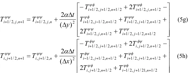
(5g)
2 / 1 , 21 / 1 , 2 / 1 2 / 1 , 2 / 1 , 2 / 1 , 2 / 1 , 2 / 1 2 / 1 , 2 / 1 , 2 / 1 2 / 1 , 2 / 1 , 2 / 1 , 2 / 1 , 2 / 1 2 , 2 / 1 , 1 , 2 / 1 ,2
2
)
(
2
n j i n j i n j i n j i n j i n j i n j i n j iT
T
T
T
T
T
x
t
T
T
(5h)Temperatures appeared in Equations (5a)-(5h) are shown in Figure (1). For more details about the discretization of this equation see [6]
Figure (1) Positions of temperatures appeared in Equations (5a) - (5h)
RESEARCH METHOD
The two-dimensional heat equation obtained from a rectangular plate
n n+ 1 n + 1/2
j – 1/2 j y t
Tj, n + 1
Tj – 1/2, n+1/2
Tj + 1/2, n+1/2 Tj,n
i+ 1/2
i
n
n +1/2 n + 1
t x
Ti+1/2,n + 1/2
Ti, n
Ti, n+ 1
Ti-1/2,n+1/2 i- 1/2
Ti,n+ 1/2
Tj,n+ 1/2
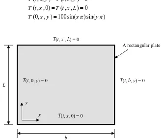
[image:4.499.101.433.83.211.2]dimension of L b, see Figure (2), along with its boundary and initial conditions can be expressed as follows:
2 2
2 2
( , 0, ) ( , , ) 0 ( , , 0) ( , , ) 0
(0, , ) 100 sin( ) sin( )
T T T
x y t
T t y T t b y
T t x T t x L
T x y x y
(6)
Figure (2) a rectangular plate L b with its boundary conditions
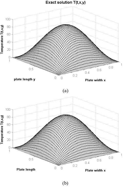
The exact solution of this equation (6) is 2
( , , ) 100 sin sin
T t x y e x y (7)
Equation (7) represents the temperature distribution which gives the value of temperature at any point within the plate and at any time. The heat conduction transferred through the wall can be then evaluated from Fourier’s law [5].
Figure (3a) shows the plot of Equation (7) while Figure (3b) shows the plot of the numerical solution obtained from the wavelet-based numerical scheme,
Equations (5a)-(5-h), both at time level t = 1 sec with time step t = 0.005 sec and
the plate is assumed to be square in shape that is L = b with spatial step x = y =
1/50.
T(t, 0, y) = 0 T(t, b, y) = 0
T(t, x, 0) = 0 T(t, x , L) = 0
b L
y
x
[image:5.499.79.413.160.446.2]ANALYSIS AND DISCUSSION
It is oblivious that the values of temperatures in Figures (3a) and (4b) are not the same. For instance, at t = 0 , the maximum value of temperature in figure (3a) that is the exact solution, is 100C occurs at the mid point of plate while the maximum value of temperature in figure (3b) that is the numerical solution obtained from the wavelet-based numerical solution is 73C which occurs at the same position.
Figure (3) the temperature distribution obtained from (a) the exact solution
(a)
[image:6.499.125.367.208.573.2]This difference in temperature values is understood as the numerical error which occurs as a result of truncating the expansion of temperature function in wavelet series. By other words, it is the difference between the derivative and difference equation based on wavelet coefficients.
The wavelet-based numerical scheme, as expected, resulted in stable solution which can be compared to the exact solution yet with an acceptable percentage of error. This unconditional stability of wavelet-based scheme represents one of the distinctive features of wavelet-based schemes based on its ability to copying with nonlinearity and large discretization meshes [3].
In wavelet-based scheme, as the time and/or special step gets larger, some of additional bases will be added to keep tracing with change of the route of curve that might result in floating points as the case of conventional explicit scheme. As a result, the numerical solution will be unaffected by the sudden change of the time and/or special step.
CONCLUSION
We now get to the conclusion that the draw back of the explicit finite difference, namely instability, has been overcome by introducing Haar wavelet analysis which, in its essence, did not influence the logical approach of that method in term of getting one temperature value in the new time step from three known temperature values obtained at the previous time step [2]. Rather, wavelet has improved this approach by self adding of new temperature values found at the middle point between the previous and next time steps (Figure 1). The same can be said concerning the special steps.
This self adding of new values can be interpreted as that wavelet analysis is built on multi-resolution analysis [3] in context of expressing a function, temperature here, in two coexist levels of resolution; the coarse level is obtained by the Haar scaling function and the other refining level is obtained by Haar wavelet function. With this, the first order of approximation by wavelet expansion, compared to the first order of approximation by Taylor expansion on which the explicit finite difference approach is based [2], will results in one unknown temperature value obtained from six known values at shorter time step. Those three extra known values will result in higher accuracy and stability scheme than the Taylor-based numerical scheme which gives one known value of temperature corresponds to three known values at longer time step.
REFERENCES
Amartunga, K. and Williams, J. R., 1994, “Wavelet-Galerkin Solutions for Two-Dimensional Partial Differential Equations”, International
Journal for Numerical Methods in Engineering, 37, pp. 2703-2716.
Carnahan, B., Luther, H. A. and Wilkes, J. O., 1969, “Applied Numerical Methods” Wiley, New York.
Daubachies, I., 1992, “Ten Lectures On Wavelets”, SIAM, Philadelphia, Pennsylvania.
Duchateau, P. and Zachmann, D., 1986, “Partial Differential Equations”, Schaum’s Outline Series, McGraw-Hill Book Company, New York
Holman, J.P., 1992, “Heat Transfer”, 7th Edition, McGraw Hill Book Company, Inc., New York.