Can Time-Varying Risk of Rare Disasters Explain
Aggregate Stock Market Volatility?
JESSICA A. WACHTER∗
ABSTRACT
Why is the equity premium so high, and why are stocks so volatile? Why are stock returns in excess of government bill rates predictable? This paper proposes an answer to these questions based on a time-varying probability of a consumption disaster. In the model, aggregate consumption follows a normal distribution with low volatility most of the time, but with some probability of a consumption realization far out in the left tail. The possibility of this poor outcome substantially increases the equity premium, while time-variation in the probability of this outcome drives high stock market volatility and excess return predictability.
THE MAGNITUDE OF THEexpected excess return on stocks relative to bonds (the equity premium) constitutes one of the major puzzles in financial economics. As Mehra and Prescott (1985) show, the fluctuations observed in the consumption growth rate over U.S. history predict an equity premium that is far too small, assuming reasonable levels of risk aversion.1One proposed explanation is that
the return on equities is high to compensate investors for the risk of a rare disaster (Rietz (1988)). An open question has therefore been whether the risk is sufficiently high, and the rare disaster sufficiently severe, to quantitatively explain the equity premium. Recently, however, Barro (2006) shows that it is possible to explain the equity premium using such a model when the probability of a rare disaster is calibrated to international data on large economic declines. While the models of Rietz (1988) and Barro (2006) advance our understanding of the equity premium, they fall short in other respects. Most importantly, these models predict that the volatility of stock market returns equals the volatility of dividends. Numerous studies show, however, that this is not the case. In fact, there is excess stock market volatility: the volatility of stock returns far
∗Jessica A. Wachter is with the Department of Finance, The Wharton School. For helpful
com-ments, I thank Robert Barro, John Campbell, Mikhail Chernov, Gregory Duffee, Xavier Gabaix, Paul Glasserman, Francois Gourio, Campbell Harvey, Dana Kiku, Bruce Lehmann, Christian Juillard, Monika Piazzesi, Nikolai Roussanov, Jerry Tsai, Pietro Veronesi, and seminar partici-pants at the 2008 NBER Summer Institute, the 2008 SED Meetings, the 2011 AFA Meetings, Brown University, the Federal Reserve Bank of New York, MIT, University of Maryland, the University of Southern California, and The Wharton School. I am grateful for financial support from the Aronson+Johnson+Ortiz fellowship through the Rodney L. White Center for Financial Research. Thomas Plank and Leonid Spesivtsev provided excellent research assistance.
1Campbell (2003) extends this analysis to multiple countries. DOI: 10.1111/jofi.12018
exceeds that of dividends (e.g., Shiller (1981), LeRoy and Porter (1981), Keim and Stambaugh (1986), Campbell and Shiller (1988), Cochrane (1992), Hodrick (1992)). While the models of Barro and Rietz address the equity premium puzzle, they do not address this volatility puzzle.
In the original models of Barro (2006), agents have power utility and the en-dowment process is subject to large and relatively rare consumption declines (disasters). This paper proposes two modifications. First, rather than being constant, the probability of a disaster is stochastic and varies over time. Sec-ond, the representative agent, rather than having power utility preferences, has recursive preferences. I show that such a model can generate volatility of stock returns close to that in the data at reasonable values of the underlying parameters. Moreover, the model implies reasonable values for the mean and volatility of the government bill rate.
Both time-varying disaster probabilities and recursive preferences are neces-sary to fit the model to the data. The role of time-varying disaster probabilities is clear; the role of recursive preferences perhaps less so. Recursive preferences, introduced by Kreps and Porteus (1978) and Epstein and Zin (1989), retain the appealing scale-invariance of power utility but allow for separation between the willingness to take on risk and the willingness to substitute over time. Power utility requires that these aspects of preferences are driven by the same parameter, leading to the counterfactual prediction that a high price–dividend ratio predicts a high excess return. Increasing the agent’s willingness to substi-tute over time reduces the effect of the disaster probability on the risk-free rate. With recursive preferences, this can be accomplished without simultaneously reducing the agent’s risk aversion.
The model in this paper allows for time-varying disaster probabilities and recursive utility with unit elasticity of intertemporal substitution (EIS). The assumption that the EIS is equal to one allows the model to be solved in closed form up to an indefinite integral. A time-varying disaster probability is modeled by allowing the intensity for jumps to follow a square-root process (Cox, Ingersoll, and Ross (1985)). The solution for the model reveals that allowing the probability of a disaster to vary not only implies a time-varying equity premium, but also increases the level of the equity premium. The dynamic nature of the model therefore leads the equity premium to be higher than what static considerations alone would predict.
the low volatility of the government bill rate because of two competing effects. When the risk of a disaster is high, rates of return fall because of precaution-ary savings. However, the probability of government default (either outright or through inflation) rises. Investors therefore require greater compensation to hold government bills.
As I describe above, adding dynamics to the rare disaster framework allows for a number of new insights. Note, however, that the dynamics in this paper are relatively simple. A single state variable (the probability of a rare disaster) drives all of the results in the model. This is parsimonious, but also unrealistic: it implies, for instance, that the price–dividend ratio and the risk-free rate are perfectly negatively correlated. It also implies a degree of comovement among assets that would not hold in the data. In SectionI.D, I suggest ways in which this weakness might be overcome while still maintaining tractability.
Several recent papers also address the potential of rare disasters to explain the aggregate stock market. Gabaix (2012) assumes power utility for the rep-resentative agent, while also assuming the economy is driven by a linearity-generating process (see Gabaix (2008)) that combines time-variation in the probability of a rare disaster with time-variation in the degree to which div-idends respond to a disaster. This set of assumptions allows him to derive closed-form solutions for equity prices as well as for prices of other assets. In Gabaix’s numerical calibration, only the degree to which dividends respond to the disaster varies over time. Therefore, the economic mechanism driving stock market volatility in Gabaix’s model is quite different from the one considered here. Barro (2009) and Martin (2008) propose models with a constant disaster probability and recursive utility. In contrast, the model considered here focuses on the case of time-varying disaster probabilities. Longstaff and Piazzesi (2004) propose a model in which consumption and the ratio between consumption and the dividend are hit by contemporaneous downward jumps; the ratio between consumption and dividends then reverts back to a long-run mean. They assume a constant jump probability and power utility. In contemporaneous independent work, Gourio (2008b) specifies a model in which the probability of a disaster varies between two discrete values. He solves this model numerically assum-ing recursive preferences. A related approach is taken by Veronesi (2004), who assumes that the drift rate of the dividend process follows a Markov switching process, with a small probability of falling into a low state. While the physical probability of a low state is constant, the representative investor’s subjective probability is time-varying due to learning. Veronesi assumes exponential util-ity; this allows for the inclusion of learning but makes it difficult to assess the magnitude of the excess volatility generated through this mechanism.
His model differs from the present one in that he assumes independent and identically distributed consumption growth (with a Bayesian agent learning about the unknown variance), and he focuses on explaining the equity premium.
Finally, this paper draws on a literature that derives asset pricing results assuming endowment processes that include jumps, with a focus on option pricing (an early reference is Naik and Lee (1990)). Liu, Pan, and Wang (2005) consider an endowment process in which jumps occur with a constant inten-sity; their focus is on uncertainty aversion but they also consider recursive utility. My model departs from theirs in that the probability of a jump varies over time. Drechsler and Yaron (2011) show that a model with jumps in the volatility of the consumption growth process can explain the behavior of im-plied volatility and its relation to excess returns. Eraker and Shaliastovich (2008) also model jumps in the volatility of consumption growth; they focus on fitting the implied volatility curve. Both papers assume an EIS greater than one and derive approximate analytical and numerical solutions. Santa-Clara and Yan (2006) consider time-varying jump intensities, but restrict attention to a model with power utility and implications for options. In contrast, the model considered here focuses on recursive utility and implications for the aggregate market.
The outline of the paper is as follows. SectionIdescribes and solves the model, SectionIIdiscusses the calibration and simulation, and SectionIIIconcludes.
I. Model
A. Assumptions
I assume an endowment economy with an infinitely lived representative agent. This setup is standard, but I assume a novel process for the endowment. Aggregate consumption (the endowment) follows the stochastic process
dCt=µCt−dt+σCt−dBt+(eZt−1)Ct−dNt, (1)
where Bt is a standard Brownian motion and Nt is a Poisson process with
time-varying intensityλt.2This intensity follows the process
dλt=κ( ¯λ−λt)dt+σλ
λtdBλ,t, (2)
whereBλ,tis also a standard Brownian motion, andBt,Bλ,t, andNtare assumed
to be independent. I assume Zt is a random variable whose time-invariant
distributionνis independent ofNt,Bt, andBλ,t. I use the notationEνto denote
expectations of functions of Zttaken with respect to the ν-distribution. Thet
subscript on Ztwill be omitted when not essential for clarity.
Assumptions (1) and (2) define Ct as a mixed jump-diffusion process. The
diffusion term µCt−dt+σCt−dBt represents the behavior of consumption in
2In what follows, all processes will be right continuous with left limits. Given a processx
t, the
normal times, and implies that, when no disaster takes place, log consumption growth over an interval t is normally distributed with mean (µ−12σ2)t and variance σ2t. Disasters are captured by the Poisson process Nt, which
allows for large instantaneous changes (“jumps”) in Ct. Roughly speaking, λt
can be thought of as the disaster probability over the course of the next year.3
In what follows, I refer to λt as either the disaster intensity or the disaster
probability depending on the context; these terms should be understood to have the same meaning. The instantaneous change in log consumption, should a disaster occur, is given by Zt. Because the focus of the paper is on disasters,
Ztis assumed to be negative throughout.
In the model, a disaster is therefore a large negative shock to consumption. The model is silent on the reason for such a decline in economic activity; ex-amples include a fundamental change in government policy, a war, a financial crisis, and a natural disaster. Given my focus on time-variation in the likeli-hood of a disaster, it is probably most realistic to think of the disaster as caused by human beings (that is, the first three examples given above, rather than a natural disaster). The recent financial crisis in the United States illustrates such time-variation: following the series of events in the fall of 2008, there was much discussion of a second Great Depression, brought on by a freeze in the financial system. The conditional probability of a disaster seemed higher, say, than in 2006.
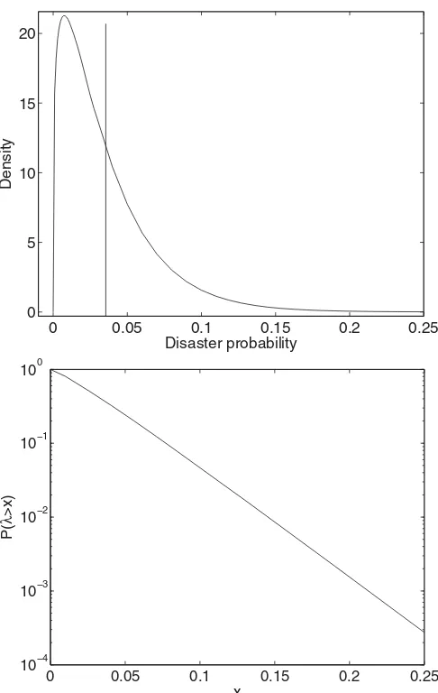
As Cox, Ingersoll, and Ross (1985) discuss, the solution to(2)has a station-ary distribution provided thatκ >0 and ¯λ >0. This stationary distribution is Gamma with shape parameter 2κλ/σ¯ λ2 and scale parameterσλ2/(2κ). If 2κλ >¯ σλ2, the Feller condition (from Feller (1951)) is satisfied, implying a finite den-sity at zero. The top panel of Figure 1 shows the probability density func-tion corresponding to the stafunc-tionary distribufunc-tion. The bottom panel shows the probability that λt exceeds x as a function of x (the y-axis uses a log scale).
That is, the panel shows the difference between one and the cumulative dis-tribution function for λt. As this figure shows, the stationary distribution of
λt is highly skewed. The skewness arises from the square root term
multi-plying the Brownian shock in (2): this square root term implies that high realizations of λt make the process more volatile, and thus further high
re-alizations more likely than they would be under a standard autoregressive process. The model therefore implies that there are times when “rare” dis-asters can occur with high probability, but that these times are themselves unusual.
I assume the continuous-time analogue of the utility function defined by Epstein and Zin (1989) and Weil (1990) that generalizes power utility to allow for preferences over the timing of the resolution of uncertainty. The continuous-time version is formulated by Duffie and Epstein (1992); I make use of a limiting
3More precisely, the probability ofkjumps over the course of a short intervaltis approximately equal toe−λtt(λtt)k
0 0.05 0.1 0.15 0.2 0.25 0
5 10 15 20
Disaster probability
Density
0 0.05 0.1 0.15 0.2 0.25 10−4
10−3 10−2 10−1 100
x
P(
λ
>x)
Figure 1. Distribution of the disaster probability,λt.The top panel shows the probability
density function forλt, the time-varying intensity (per year) of a disaster. The solid vertical line is located at the unconditional mean of the process. The bottom panel shows the probability that
λexceeds a valuex, forxranging from zero to 0.25. They-axis on the bottom panel uses a log (base–10) scale.
case of their model that sets the parameter associated with the intertemporal elasticity of substitution equal to one. Define the utility function Vt for the
representative agent using the following recursion:
Vt=Et
∞
t
where
f(C,V)=β(1−γ)V
logC− 1
1−γ log((1−γ)V)
. (4)
Note that Vt represents continuation utility, that is, utility of the future
con-sumption stream. The parameter β is the rate of time preference. I follow common practice in interpretingγ as relative risk aversion. Asγ approaches one,(4)can be shown to be ordinally equivalent to logarithmic utility. I assume throughout that β >0 andγ >0. Most of the discussion focuses on the case γ >1.
B. The Value Function and the Risk-Free Rate
Let W denote the wealth of the representative agent and J(W, λ) the value function. In equilibrium, it must be the case thatJ(Wt, λt)=Vt. Conjecture that
the price–dividend ratio for the consumption claim is constant. In particular, letStdenote the value of a claim to aggregate consumption. Then
St
Ct
=l (5)
for some constantl.4The process for consumption and the conjecture(5)imply
thatStsatisfies
dSt=µSt−dt+σSt−dBt+(eZt−1)St−dNt. (6)
Letrtdenote the instantaneous risk-free rate.
To solve for the value function, consider the Hamilton–Jacobi–Bellman equa-tion for an investor who allocates wealth between St and the risk-free asset.
Letαtbe the fraction of wealth in the risky assetSt, and (with some abuse of
notation) letCtbe the agent’s consumption. Wealth follows the process
dWt=(Wt−αt(µ−rt+l−1)+Wt−rt−Ct−)dt+Wt−αtσdBt+αt(eZt−1)Wt−dNt.
Optimal consumption and portfolio choice must satisfy the following (Duffie and Epstein (1992)):
sup
αt,Ct
JW(Wtαt(µ−rt+l−1)+Wtrt−Ct)+Jλκ( ¯λ−λt)+
1 2JW WW
2 tα
2 tσ
2
+1
2Jλλσ
2
λλt+λtEν[J(Wt(1+αt(eZt−1)), λt)
−J(Wt, λt)]+ f(Ct,J)
=0, (7)
4Indeed, the fact thatSt/C
tis constant (and equal to 1/β) arises from the assumption of unit
where Ji denotes the first derivative of J with respect to i, for i equal to λ
or W, and Ji j the second derivative of J with respect to i and j. Note that
the instantaneous return on wealth invested in the risky asset is determined by the dividend yieldl−1as well as by the change in price. Note also that the
instantaneous expected change in the value function is given by the continuous drift plus the expected change due to jumps.
As AppendixA. I shows, the form of the value function and the envelope condi-tion fC=JW imply that that the wealth–consumption ratiol=β−1. Moreover,
the value function takes the form
J(W, λ)= W 1−γ
1−γI(λ). (8)
The functionI(λ) is given by
I(λ)=ea+bλ, (9)
where
a= 1−γ
β
µ−1
2γ σ
2
+(1−γ) logβ+bκλ¯
β , (10)
b= κ+β
σλ2 −
κ+β
σλ2
2
−2Eν[e
(1−γ)Z−1]
σλ2 . (11)
It follows from (11) that, for γ >1, b>0.5 Therefore, by (8), an increase in
disaster risk reduces utility for the representative agent. As SectionI.Dshows, the price of the dividend claim falls when the disaster probability rises. The agent requires compensation for this risk (because utility is recursive, marginal utility depends on the value function), and thus time-varying disaster risk increases the equity premium.
AppendixA.Ishows that the risk-free rate is given by
rt=β + µ − γ σ2
standard model
+ λtEν[e−γZ(eZ−1)]
disaster risk
. (12)
The term above the first bracket in(12)is the same as in the standard model without disaster risk; β represents the role of discounting, µ intertemporal smoothing, andγprecautionary savings. The term multiplyingλtin(12)arises
from the risk of a disaster. BecauseeZ<1, the risk-free rate is decreasing in
λ. An increase in the probability of a rare disaster increases the representative agent’s desire to save, and thus lowers the risk-free rate. The greater is risk aversion, the greater is this effect.
0 0.02 0.04 0.06 0.08 0.1 −0.08
−0.06 −0.04 −0.02 0 0.02 0.04
Expected return
Disaster probability government bill expected return government bill yield
risk−free rate
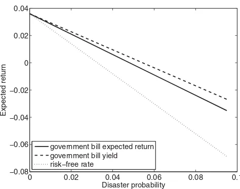
Figure 2. Government bill return in the time-varying disaster risk model.This figure
showsrb, the instantaneous expected return on a government bill;rL, the instantaneous expected
return on the bill conditional on no default; andr, the rate of return on a default-free security as functions of the disaster intensityλ. All returns are in annual terms.
C. Risk of Default
Disasters often coincide with at least a partial default on government secu-rities. This point is of empirical relevance if one tries to match the behavior of the risk-free asset to the rate of return on government securities in the data. I therefore allow for partial default on government debt, and consider the rate of return on this defaultable security. I assume that, in the event of disaster, there will be a default on government liabilities with probability q. I follow Barro (2006) in assuming that, in the event of default, the percentage loss is equal to the percentage decline in consumption.
Specifically, let rL
t denote the interest rate that investors would receive if
default does not occur. As shown in Appendix A.V, the equilibrium relation betweenrL
t andrtis
rtL=rt+λtqEν[e−γZt(1−eZ)]. (13)
Let rb denote the instantaneous expected return on government debt. Then
rb
t =rtL+λtqEν[eZ−1], so
rtb=rt+λtqEν[(e−γZt−1)(1−eZ)]. (14)
The second term in (14) has the interpretation of a disaster risk premium: the percentage change in marginal utility is multiplied by the percentage loss on the asset. An analogous term will appear in the expression for the equity premium below. Figure 2 shows the face value of government debt, rL
t, the
instantaneous expected return on government debtrb
rtas a function ofλt. Because of the required compensation for default,rtLlies
abovert. The expected return lies between the two because the actual cash
flow that investors receive from the government bill will be belowrL
t if default
occurs.
All three rates decrease inλt because, at these parameter values, a higher
λt induces a greater desire to save. However,rtL and rtb are less sensitive to
changes inλthanrtbecause of an opposing effect: the greater isλt, the greater
is the risk of default and therefore the greater the return investors demand for holding the government bill. Because of a small cash flow effect,rtbdecreases more thanrtL, but still less thanrt.
D. The Dividend Claim
This section describes prices and expected returns on the aggregate stock market. Let Dt denote the dividend. I model dividends as levered
consump-tion, that is, Dt=Ctφ as in Abel (1999) and Campbell (2003). Ito’s Lemma
implies
dDt
Dt−
=µDdt+φσdBt+(eφZt−1)dNt, (15)
whereµD=φµ+12φ(φ−1)σ2. Forφ >1, dividends fall by more than
consump-tion in the event of a disaster. This is consistent with the U.S. experience (for which accurate data on dividends are available) as discussed in Longstaff and Piazzesi (2004).
While dividends and consumption are driven by the same shocks,(15)does allow dividends and consumption to wander arbitrarily far from one another. This could be avoided by modeling the consumption–dividend ratio as a sta-tionary but persistent process, as in, for example, Lettau and Ludvigson (2005), Longstaff and Piazzesi (2004), and Menzly, Santos, and Veronesi (2004). In or-der to focus on the novel implications of time-varying disaster risk, I do not take this route here.
It is convenient to price the claim to aggregate dividends by first calculat-ing the state-price density. Unlike the case of time-additive utility, the case of recursive utility implies that the state-price density depends on the value func-tion. In particular, Duffie and Skiadas (1994) show that the state-price density πtis equal to
πt=exp
t
0
fV(Cs,Vs)ds
fC(Ct,Vt), (16)
where fC and fV denote derivatives of f with respect to the first and second
argument, respectively.
LetFt=F(Dt, λt) denote the price of the claim to future dividends. Absence of
using the state-price density:
Define a function representing a single term in this integral:
H(Dt, λt,s−t)=Et
to the dividend paidτ years in the future. AppendixA.IIIshows thatH takes a simple exponential form,
AppendixA.IIIdiscusses further properties of interest, such as existence, sign, and convergence asτapproaches infinity. In particular, forφ >1,aφ(τ) andbφ(τ)
are well defined for all values ofτ. Moreover,bφ(τ) is negative. The sign ofbφ(τ)
is of particular importance for the model’s empirical implications. Negative bφ(τ) implies that, when risk premia are high (namely, when disaster risk is
high), valuations are low. Thus, the price–dividend ratio (which is F(D, λ, τ) divided by the aggregate dividend D) predicts realized excess returns with a negative sign.
ratio (Campbell and Shiller (1988)), the net effect depends on the interplay of three forces: the effect of the disaster risk on risk premia, on the risk-free rate, and on future cash flows. A precise form of this statement is given in SectionI.F. The result thatbφ(τ) is negative implies that, indeed, the risk premium and
cash flow effect dominate the risk-free rate effect. Thus, the price–dividend ratio will predict excess returns with the correct sign. AppendixA.III shows that this result holds generally under the reasonable condition that φ >1. Section I.G contrasts this result with what holds in a dynamic model with power utility.
The results in this section also suggest the following testable implication: stock market valuations should fall when the risk of a rare disaster rises. The risk of a rare disaster is unobservable, but, given a comprehensive data set, one can draw conclusions based on disasters that have actually occurred. This is important because it establishes independent evidence for the mechanism in the model.
Specifically, Barro and Ursua (2009) address the question: given a large de-cline in the stock market, how much more likely is a dede-cline in consumption than otherwise? Barro and Ursua augment the data set of Barro and Ursua (2008) with data on national stock markets. They look at cumulative multi-year returns on stocks that coincide with macroeconomic contractions. Their sample has 30 countries and 3,037 annual observations; there are 232 stock market crashes (defined as cumulative returns of –25%) and 100 macroeco-nomic contractions (defined as the average of the decline in consumption and GDP). There is a 3.8% chance of moving from “normalcy” into a state with a contraction of 10% or more. This number falls to 1% if one conditions on a lack of a stock market crash. If one considers major depressions (defined as a de-cline in fundamentals of 25% or more), there is a 0.89% chance of moving from normalcy into a depression. Conditioning on no stock market crash reduces the probability to 0.07%.
Also closely related is recent work by Berkman, Jacobsen, and Lee (2011), who study the correlation between political crises and stock returns. Berk-man, Jacobsen, and Lee make use of the International Crisis Behavior (ICB) database, a detailed database of international political crises occurring during the period 1918 to 2006. Rather than dating the start of a crisis with a military action itself, the database identifies the start of a crisis with a change in the probability of a threat.6A regression of the return on the world market on the
number of such crises in a given month yields a coefficient that is negative and statistically significant. Results are particularly strong for the starting year of a crisis, for violent crises, and for crises rated as most severe. The authors also find a statistically significant effect on valuations: the correlation between the number of crises and the earnings–price ratio on the S&P 500 is positive and statistically significant, as is the correlation between the crisis severity index and the earnings–price ratio. Similar results hold for the dividend yield.
Comparing the results in this section and in SectionI.Bindicate that both the risk-free rate and the price–dividend ratio are driven by the disaster probabilityλt; this follows from the fact that there is a single state variable.
This perfect correlation could be broken by assuming that consumption is sub-ject to two types of disaster, each with its own time-varying intensity, and further assuming that one type has a stronger effect on dividends (as modeled through highφ) than the other. The real interest rate and the price–dividend ratio would be correlated with both intensities, but to different degrees, and thus would not be perfectly correlated with one another. The correlation between nominal rates and the price–dividend ratio could be further reduced by introducing a third type of consumption disaster. The three types could differ across two dimensions: the impact on dividends and the impact on expected in-flation. The expected inflation process would affect the prices of nominal bonds but would not (directly) affect stocks. I conjecture that the generalized model could be constructed to be as tractable as the present one.
E. The Equity Premium
The equity premium arises from the comovement of the agent’s marginal utility with the price process for stocks. There are two sources of this comove-ment: comovement during normal times (diffusion risk), and comovement in times of disaster (jump risk). Ito’s Lemma implies that Fsatisfies
dFt
Ft−
=µF,tdt+σF,t[dBtdBλ,t]⊤+(eφZ−1)dNt, (21)
for processesµF,tandσF,t. It is helpful to define notation for the price–dividend
ratio. Let
G(λ)=
∞
0
exp{aφ(τ)+bφ(τ)λ}dτ. (22)
Then
σF,t=[φσ (G′(λt)/G(λt))σλ
λt]. (23)
Ito’s Lemma also implies
dπt
πt−
=µπ,tdt+σπ,t[dBtdBλ,t]⊤+(e−γZt−1)dNt, (24)
where
σπ,t=[−γ σ bσλ
λt] (25)
as shown in AppendixA.II. Finally, define
rte=µF,t+
Dt
Ft
Thenre
t can be understood to be the instantaneous return on equities.7 The
instantaneous equity premium is thereforere t −rt.
AppendixA.IVshows that the equity premium can be written as
rte−rt= −σπ,tσF⊤,t+λtEν[(e−γZ−1)(1−eφZ)]. (27)
The first term represents the portion of the equity premium that is compensa-tion for diffusion risk (which includes time-varyingλt). The second term is the
compensation for jump risk. While the diffusion term represents the comove-ment between the state-price density and prices during normal times, the jump risk term shows the comovement between the state-price density and prices during disasters. That is,
for a timetsuch that a jump takes place. Substituting(23)into(27)implies
rte−rt= φγ σ2
The first and third terms are analogous to expressions in Barro (2006): the first term is the equity premium in the standard model with normally distributed consumption growth, while the third term arises from the (static) risk of a disaster. The second term is new to the dynamic model. This is the risk premium due to time-variation in disaster risk. Becausebφis negative,G′is also negative.
Moreover, bis positive, so this term represents a positive contribution to the equity premium. Because both the second and the third terms are positive, an increase in the risk of rare disaster increases the equity premium.8
The instantaneous equity premium relative to the government bill rate is equal to(28)minus the default premiumrb
t −rt(given in(14)):
7The first term in(26)is the percentage drift in prices, the second term is the instantaneous dividend yield, and the third term is the expected decline in prices in the event of a disaster. The first plus the third term constitutes the expected percentage change in prices.
0 0.02 0.04 0.06 0.08 0.1 0
0.02 0.04 0.06 0.08 0.1 0.12 0.14 0.16 0.18 0.2
Risk premium
Disaster probability standard model
static disaster risk time−varying disaster risk
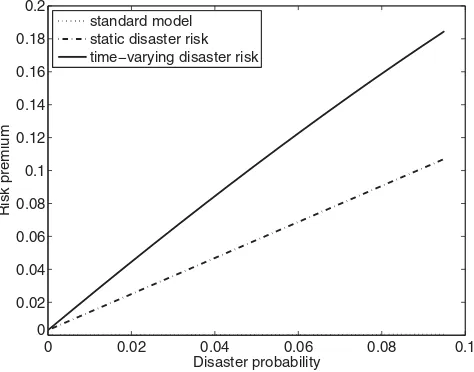
Figure 3. Decomposition of the equity premium in the time-varying disaster risk model.
The solid line shows the instantaneous equity premium (the expected excess return on equity less the expected return on the government note), the dashed line shows the equity premium in a static model with disaster risk, and the dotted line shows what the equity premium would be if disaster risk were zero.
The last term in (29) takes the usual form for the disaster risk premium: the percentage change in marginal utility is multiplied by the percentage loss. Here, with probabilityq, the expected loss on equity relative to bonds is reduced because both assets perform poorly. This instantaneous equity premium is shown in Figure3(solid line). The difference between the dashed line and the solid line represents the component of the equity premium that is new to the dynamic model, and shows that this term is large. The dotted line represents the equity premium in the standard diffusion model without disaster risk and is negligible compared with the disaster risk component. Figure3shows that the equity premium is increasing with the disaster risk probability.
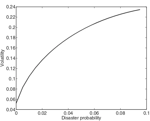
Equation(29)and Figure3show that the return required for holding equity increases with the probability of a disaster. How does it depend on a more traditional measure of risk, namely, the equity volatility? When there is no disaster, instantaneous volatility can be computed directly from(23):
σF,tσF⊤,t
1 2 =
φ2σ2+
G′(λ
t)
G(λt)
2 σλ2λt
1 2 .
0 0.02 0.04 0.06 0.08 0.1 0.04
0.06 0.08 0.1 0.12 0.14 0.16 0.18 0.2 0.22 0.24
Volatility
Disaster probability
Figure 4. Equity volatility in the time-varying disaster risk model.The figure shows
in-stantaneous equity return volatility as a function of the disaster probabilityλt. All quantities are in annual terms.
falls when the disaster probability increases, the model is consistent with the “leverage effect” found by Black (1976), Schwert (1989), and Nelson (1991).
The above equations show that an increase in the equity premium is accom-panied by an increase in volatility. The net effect of a change inλon the Sharpe ratio (the equity premium divided by the volatility) is shown in Figure5. Bad times, interpreted in this model as times with a high probability of disaster, are times when investors demand a higher risk-return tradeoff than usual. Har-vey (1989) and subsequent papers report empirical evidence that the Sharpe ratio indeed varies countercyclically. Like the model of Campbell and Cochrane (1999), this model is consistent with this evidence.
The time-varying disaster risk model generates a countercyclical Sharpe ratio through two mechanisms. First, the value function varies withλt: when
disaster risk is high, investors require a greater return on all assets with prices negatively correlated withλ. The component of the equity premium associated with time-varyingλtthus rises linearly withλwhile volatility rises only with
the square root. Second, the component of the equity premium corresponding to disaster risk itself (the last term in(29)) has no counterpart in volatility. This term compensates equity investors for negative events that are not captured by the standard deviation of returns.
F. Zero-Coupon Equity
0 0.02 0.04 0.06 0.08 0.1 0
0.1 0.2 0.3 0.4 0.5 0.6 0.7 0.8
Sharpe ratio
Disaster probability
Figure 5. Sharpe ratio in the time-varying disaster risk model.This figure shows the
in-stantaneous equity premium over the government bill divided by the inin-stantaneous equity return volatility (the Sharpe ratio) as a function of disaster probabilityλt. All quantities are in annual terms.
Recall that
H(Dt, λt,T −t)=exp
aφ(τ)+bφ(τ)λt
Dt
is the time-tprice of the claim that pays the aggregate dividend at timet+τ. Appendix A.III shows that the risk premium on the zero-coupon claim with maturityτ is equal to
re,(τ)
t −rt=φγ σ2−λtσλ2bφ(τ)b+λtEν[(e−γZ−1)(1−eφZ)]. (30)
Like the equity premium, the risk premium on zero-coupon equity is positive and increasing inλt.
Zero-coupon equity can help answer the question of why the price–dividend ratio on the aggregate market is decreasing inλt. Becausebφ(0)=0, the
ques-tion can be restated as: why isb′
φ(τ) negative for small values ofτ?
9The
differ-ential equation forbφ(τ) is given by(A27). Evaluating at zero yields:
b′
φ(0)=Eν[e(φ−γ)Z−e(1−γ)Z]= −Eν[e−γZ(eZ−1)]
risk-free rate
−Eν[(e−γZ−1)(1−eφZ)]
equity premium
+ Eν[eφZ−1]
expected future dividends
. (31)
9Note thatb
φ(τ) is monotonically decreasing. This follows from the fact that, asτ increases,
Equation(31)shows that the change inbφ(τ) can be written in terms of risk
premium, risk-free rate, and cash flow effects. The first term multipliesλtin
the equation for the risk-free rate (12). The second term multipliesλt in the
equation for the risk premium(30)in the limit asτ approaches zero. The third term represents the effect of a change inλton expected future dividends:eφZ−1
is the percentage change in dividends in the event of a disaster. The terms corresponding to the risk-free rate and the risk premium enter with negative signs, because higher discount rates reduce the price. Expected future dividend growth enters with a positive sign because higher expected cash flows raise the price. Indeed, the term corresponding to the equity premium and to expected future dividends together exceeds that of the risk-free rate whenφ >1.
As explained in the paragraph above, understandingb′
φ(τ) for low values of τ is sufficient for understanding why the price–dividend ratio is a decreasing function of λt. However, it is also instructive to decompose b′φ(τ) for general
values ofτ. At longer maturities, it is possible forλtto change before the claim
matures. Thus, there are additional terms that account for the effect of future changes inλt:
The first three terms in this more general decomposition are analogous to those in the simpler(31). The final two terms account for the effect of future changes in λt. The first of these is a Jensen’s inequality term: all else equal, more
volatility in the state variable increases the price–dividend ratio. The second of these represents the fact that, ifλtis high in the present,λtis likely to decrease
in the future on account of mean reversion.
While the focus of this paper is on the aggregate market, it is also of interest to compare the model’s implications for zero-coupon equity to the behavior of these claims in the data.10van Binsbergen, Brandt, and Koijen (2012) use option price
data to calculate prices and risk premia on zero-coupon equity. Their methods are able to establish prices for dividend claims that have variable maturities of less than 2 years. They find that these claims have expected excess returns that are statistically different from zero. In other words, the equity premium arises at least in part from the short-term portion of the dividend stream. van Binsbergen, Brandt, and Koijen argue that this evidence is contrary to
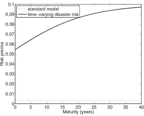
0 5 10 15 20 25 30 35 40 0
0.01 0.02 0.03 0.04 0.05 0.06 0.07 0.08 0.09 0.1
Risk premia
Maturity (years) standard model
time−varying disaster risk
Figure 6. Risk premia on zero-coupon equity. This figure shows average risk premia on
zero-coupon equity claims as a function of maturity. Zero-coupon equity is a claim to the aggregate dividend at a single point in time (referred to as the maturity). Risk premia are defined as expected excess returns less the risk-free rate. The dotted line shows what risk premia would be if the disaster risk were zero. The solid line shows risk premia in the model. Risk premia are expressed in annual terms.
the implications of some leading asset pricing models such as Bansal and Yaron (2004) and Campbell and Cochrane (1999). In these models, the claim to dividends in the very near future has a premium close to zero; the equity premium arises from dividends paid in the far future.
In contrast, the present model implies a substantial equity premium for the short-term claim, and thus is consistent with the empirical evidence. Figure6
plots risk premia (30)as a function of maturity. While the equity premium is increasing in maturity (that is, the “term structure of equities” is upward-sloping), the intercept of the graph is not at zero but rather at 5.5%. The reason is that a major source of the equity premium is disaster risk itself. Equities of all maturities have equal exposure to this risk, and thus even equities with short maturities have substantial risk premia, as the data imply.11
G. Comparison with Power Utility
To understand the role played by the recursive utility assumption, it is in-structive to consider the properties of a model with time-varying disaster risk
and time-additive utility.12 Consider a model with identical dynamics of
con-sumption and dividends, but where utility is given by
Vt=Et
AppendixCshows that the risk-free rate under this model is equal to
rt=β+γ µ−
1
2γ(γ+1)σ
2−λ
tEν[e−γZ−1], (32)
the equity premium is given by
re
t −rt=φγ σ2+λtEν[(e−γZ−1)(1−eφZ)], (33)
and the value of the aggregate market takes the form
F(Dt, λt)=Dt
The functionsap,φ(τ) and bp,φ(τ) satisfy ordinary differential equations given
in AppendixC. The solutions are
ap,φ(τ)=
It is useful to contrast(35)with its counterpart in the recursive utility model. Under recursive utility, bφ(τ) is negative forφ >1, implying that the price–
dividend ratio is decreasing in λt. For power utility,bφ(τ) is negative only if φ > γ; otherwise it is positive.13 Under the reasonable assumption thatφ is
less thanγ, the power utility model makes the counterfactual prediction that price–dividend ratios predict excess returns with a positive sign.14
What accounts for the difference between the power utility model and the recursive utility model? The answer lies in the behavior of the risk-free rate. Comparing (32)with (12) reveals that the risk-free rate under power utility falls more in response to an increase in disaster risk than under recursive utility with EIS equal to one. In the power utility model, the risk-free rate effect exceeds the combination of the equity premium and cash flow effects, and, as a result, the price–dividend ratio increases with disaster risk.15
II. Calibration and Simulation
A. Calibration
A.1. Distribution of Consumption Declines
The distribution of the percentage decline, 1−eZ, is taken directly from the
data . That is, 1−eZis assumed to have a multinomial distribution, with
out-comes given by actual consumption declines in the data. I use the distribution of consumption declines found by Barro and Ursua (2008). Barro and Ursua update the original cross-country data set of Maddison (2003) used by Barro (2006). The Maddison data consist of declines in GDP; Barro and Ursua cor-rect errors and fill in gaps in Maddison’s GDP data, as well as construct an analogous data set of consumption declines. I calibrate to the consumption data because it is a more appropriate match to consumption in the model than is GDP. However, results obtained from GDP data are very similar. The fre-quency of large consumption declines implies an average disaster probability,
¯
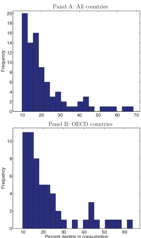
λ, of 3.55%.16The distribution of consumption declines in Panel A of Figure7
comes from data on 22 countries from 1870 to 2006. One possible concern about the data is the relevance of this group for the United States. For this reason, Barro and Ursua (2008) also consider the disaster distribution for a subset consisting of developed countries. For convenience, I follow Barro and Ursua
14Gabaix (2012) solves a model with disaster risk and power utility assuming linearity gener-ating processes for consumption and dividends. While the theoretical model that Gabaix proposes allows for a time-varying probability of rare disasters, the disaster probability is assumed to be constant in the calibration and dynamics are generated by changing the degree to which divi-dends respond to a consumption disaster. As this discussion shows, incorporating time-varying probabilities into Gabaix’s calibrated model would likely reduce the model’s ability to match the data.
15As in the recursive utility model, examiningb′
p,φ(0) allows a precise statement of these trade-offs. For power utility:
b′
p,φ(0)= Eν[e(φ−γ)Z−1]
= −Eν[e−γZ−1]
risk-free rate
−Eν[(e−γZ−1)(1−eφZ)]
equity premium
+ Eν[eφZ−1]
expected future dividends
,
which is greater than zero whenγ > φ.
10 20 30 40 50 60 70 0
2 4 6 8 10 12 14 16 18 20
Frequency
10 20 30 40 50 60
0 2 4 6 8 10
Percent decline in consumption
Frequency
Panel A: All countries
Panel B: OECD countries
Figure 7. Distribution of consumption declines in the event of a disaster. Histograms
show the distribution of large consumption declines (in percentages). Panel A shows data for 22 countries, 17 of which are OECD countries and 5 of which are not; Panel B shows data for the subsample of OECD countries. Data are from Barro and Ursua (2008). Panel A is the distribution of 1−eZin the baseline calibration, while Panel B is the distribution of 1−eZin the calibration
for OECD countries.
and refer to these as “OECD countries.”17 The distribution of consumption declines in these economies is given in Panel B. There are fewer of such crises;
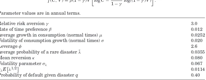
Table I
Parameters for the Time-Varying Disaster Risk Model
The table shows parameter values for the time-varying disaster risk model. The process for the disaster intensity is given by
dλt=κ( ¯λ−λt)dt+σλ
λtdBλ,t.
The consumption (endowment) process is given by
dCt=µCtdt+σCtdBt+(eZt−1)Ct−dNt,
whereNt is a Poisson process with intensityλt, and Ztis calibrated to the distribution of large
declines in GDP in the data. The dividendDtequalsCtφ. The representative agent has recursive
utility defined byVt=Et
∞
t f(Cs,Vs)ds, with normalized aggregator
f(C,V)=β(1−γ)V
logC− 1
1−γ log((1−γ)V)
.
Parameter values are in annual terms.
Relative risk aversionγ 3.0
Rate of time preferenceβ 0.012
Average growth in consumption (normal times)µ 0.0252 Volatility of consumption growth (normal times)σ 0.020
Leverageφ 2.6
Average probability of a rare disaster ¯λ 0.0355
Mean reversionκ 0.080
Volatility parameterσλ 0.067
σλE
λ1/2
0.0114
Probability of default given disasterq 0.40
the implied average disaster probability is 2.86%. However, eliminating the non-OECD crises in effect eliminates many comparatively minor crises (gen-erally occurring after World War II). The overall distribution is shifted toward the more serious crises. In what follows, I use the distribution in Panel A for the base calibration, while the implications of the distribution in Panel B are explored in SectionII.D.
A.2. Other Parameters
TableIdescribes model parameters other than the disaster distribution de-scribed above. Results are compared with quarterly U.S. data beginning in 1947 and ending in the first quarter of 2010. Equities are constructed using the CRSP value-weighted index, while the risk-free rate moments are con-structed from real returns on the 3-month Treasury bill. Postwar data are chosen as the comparison point in order to provide a clean comparison to mo-ments of the model that are calculated conditional on no disasters having occurred. Two types of moments are simulated from the model. The first type
(referred to as “population” in the tables) is calculated based on all years in the simulation. The second type (referred to as “conditional” in the tables) is calculated after first eliminating years in which one or more disasters took place.18
In the model, time is measured in years and parameter values should be interpreted accordingly. The drift rateµis calibrated so that, in normal periods, the expected growth rate of log consumption is 2.5% per annum.19The standard
deviation of log consumptionσ is 2% per annum. These parameters are chosen as in Barro (2006) to match postwar data in G7 countries. The probability of default given disaster,q, is set equal to 0.4, calculated by Barro based on data for 35 countries over the period 1900 to 2000.
Barro and Ursua (2008) consider values of risk aversion equal to 3.0 and 3.5; because the dynamic nature of the present model leads to a higher risk premium, I use risk aversion equal to three. Given these parameter choices, a rate of time preference (β) equal to 1.2% per annum matches the average real return on the 3-month Treasury bill in postwar U.S. data.
Leverage,φ, is set equal to 2.6; this is a conservative value by the standards of prior literature. For example, the model of Bansal and Yaron (2004) uses leverage parameters of three and five. The ratio of dividend to consumption volatility in postwar U.S. data is 4.9. In the present model, φ has implica-tions for the response of dividends to a disaster, relative to consumption. For example, if consumption falls by 40%, dividends fall by 1−0.62.6=74%. Is
this reasonable? For many countries and events in the Barro and Ursua data set, accurate dividend and earnings information is difficult to come by. How-ever, data on corporate earnings are available for the Great Depression, as described by Longstaff and Piazzesi (2004), who argue that earnings may be a better proxy for economic dividends due to artificial dividend smoothing. Longstaff and Piazzesi report that, in the first year of the Great Depression, when consumption fell by 10%, corporate earnings fell by more than 103%. In their calibration, they adopt a more conservative assumption: for a 10% decline in consumption, earnings fall by 90%. This is consistent with a lever-age parameter of 22. However, the Longstaff and Piazzesi calibration assumes that the consumption–dividend ratio is stationary; thus, not all of the dividend decline is permanent. One approach to this issue would be to model a sta-tionary consumption–dividend ratio. As argued above, this would complicate the model significantly, so instead I adopt a relatively conservative value for leverage along with the simpler assumption that the dividend decline, like the consumption decline, is permanent.
Other novel parameters are (implicitly) the EIS, the mean reversion of the disaster intensity, κ, and the volatility parameter for the disaster intensity, σλ. The EIS is set equal to one for tractability. A number of studies conclude
18For calculations done over consecutive years, relevant periods are omitted. For example, for evaluating predictability over 10-year horizons, 10-year periods of the simulation with a disaster are omitted.
Table II
Population Moments from Simulated Data and Sample Moments from the Historical Time Series
The model is simulated at a monthly frequency and simulated data are aggregated to an annual frequency. Data moments are calculated using overlapping annual observations constructed from quarterly U.S. data, from 1947 through the first quarter of 2010. With the exception of the Sharpe ratio, moments are in percentage terms. The second column reports population moments from simulated data. The third column reports moments from simulated data that are calculated over years in which a disaster did not occur. The last column reports annual sample moments. Rb
denotes the gross return on the government bond,Rethe gross equity return,cgrowth in log
consumption, anddgrowth in log dividends.
Model
Population Conditional U.S. Data
E[Rb] 0.99 1.36 1.34
σ(Rb) 3.79 2.00 2.66
E[Re−Rb] 7.61 8.85 7.06
σ(Re) 19.89 17.66 17.72
Sharpe Ratio 0.39 0.49 0.40
σ(c) 6.36 1.99 1.34
σ(d) 16.53 5.16 6.59
that reasonable values for this parameter lie in a range close to one, or slightly lower than one (e.g., Vissing-Jørgensen (2002)). Mean reversion κ is chosen to match the annual autocorrelation of the price–dividend ratio in postwar U.S. data. Because λt is the single state variable, the autocorrelation of the
price–dividend ratio implied by the model is determined almost entirely by the autocorrelation ofλt. Settingκequal to 0.080 generates an autocorrelation
for the price–dividend ratio equal to 0.92, its value in the data. The volatil-ity parameter σλ is chosen to be 0.067; as discussed below, this generates a
reasonable level of volatility in stock returns. The table also reportsσλE[λ1/2],
which is a measure of the annual volatility ofλt. This measure indicates that
λtvaries (approximately) by 1.14 percentage points a year. That is, whenλtis
one standard deviation above its mean, its value is 4.49%.
B. Simulation Results
TableII describes moments from a simulation of the model as well as mo-ments from postwar U.S. data. The model is discretized using an Euler ap-proximation (see (Glasserman, 2004, Chap. 3)) and simulated at a monthly frequency for 50,000 years; simulating the model at higher frequencies pro-duces negligible differences in the results.20First, I simulate the seriesλ
tand
logCt. Given the simulated series λt, the price–dividend ratio is given by
(22)and the yield on government debt,rL
t, is given by(13). Equity returns are
computed using the series for the price–dividend ratio and for consumption growth, while bond returns are computed using(A41). The resulting series for monthly returns and growth rates in fundamentals are then compounded to an annual frequency.
The model can be rejected if it offers unrealistic implications for the mean and volatility of the aggregate market, Treasury bills, and consumption and dividend growth as well as for predictability of stock returns and consumption growth.21These particular measures have been the focus of much of the recent
asset pricing literature. As I argue below, the model’s implications are in fact realistic. TableIIshows that the model generates a realistic equity premium. In population, the equity premium is 7.6%, while conditional on no disasters it is 8.9%. In the historical data the equity premium is 7.1%. The expected return on the government bill is 1% in population, 1.36% conditional on no disasters, and 1.34% in the data. The model predicts equity volatility of 19.9% per annum in population and 17.7% conditional on no disasters. The observed volatility is 17.7%. The Sharpe ratio is 0.39 in population, 0.49 conditional on no disasters, and 0.40 in the data.
The model is able to generate reasonable volatility for the stock market with-out generating excessive volatility for the government bill or for consumption and dividends. Note that the parameter values are not explicitly chosen to tar-get a low interest rate volatility. The volatility of the government bill is 3.8% in population, much of which is due to realized disasters; it is 2.0% conditional on no disasters. This compares with a volatility of 2.7% in the data. Given that interest rate volatility in the data arises largely from unexpected inflation that is not captured by the model, the data volatility should be viewed as an upper bound on reasonable model volatility.
The volatilities for consumption and dividends predicted by the model for pe-riods of no disasters are also below their data counterparts. Conditional on no disasters, consumption volatility is 2.0%, compared with 1.3% in the data. Divi-dend volatility is 5.2%, compared with 6.6% in the data. Including rare disasters in the data simulated from the model has a large effect on dividend volatility. When the disasters are included, dividend volatility is 16.5%. The difference be-tween the effect of including rare disasters on returns as compared with the ef-fect on fundamentals is striking. Unlike dividends, returns exhibit a relatively small difference in volatility when calculated with and without rare disasters: 19.9% versus 17.7%. This is because a large amount of the volatility in returns arises from variation in the equity premium. Risk premia are equally variable regardless of whether disasters actually occur in the simulated data or not.
I next discuss the model’s implications for excess return and consumption predictability. These moments are not explicit targets of the calibration, but follow naturally given the model’s properties, as described in Section I.D. Table III reports the results of regressing long-horizon excess returns (the
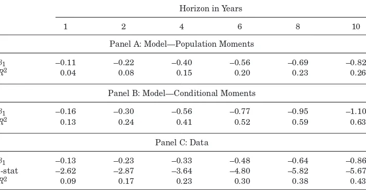
Table III
Long-Horizon Regressions: Excess Returns
Excess returns are regressed on the lagged price–dividend ratio in data simulated from the model and in quarterly data from 1947 to 2010.1. The table reports predictive coefficients (β1);R2 statis-tics; and, for the sample, Newey–Westt-statistics for regressions
h
i=1 logRe
t+i
−logRb t+i
=β0+β1(pt−dt)+ǫt.
Here,Ret+iandRbt+iare, respectively, the return on the aggregate market and the return on the government bill betweent+i−1 andt+i, and pt−dt is the log price–dividend ratio on the
aggregated market. The time-varying disaster risk model is simulated at a monthly frequency and simulated data are aggregated to an annual frequency. Panel A reports population moments from simulated data. Panel B reports moments from simulated data that are calculated over years in which a disaster does not take place (for a horizon of two, for example, all 2-year periods in which a disaster takes place are eliminated). Panel C reports sample moments.
Horizon in Years
1 2 4 6 8 10
Panel A: Model—Population Moments
β1 –0.11 –0.22 –0.40 –0.56 –0.69 –0.82
R2 0.04 0.08 0.15 0.20 0.23 0.26
Panel B: Model—Conditional Moments
β1 –0.16 –0.30 –0.56 –0.77 –0.95 –1.10
R2 0.13 0.24 0.41 0.52 0.59 0.63
Panel C: Data
β1 –0.13 –0.23 –0.33 –0.48 –0.64 –0.86
t-stat –2.62 –2.87 –3.64 –4.80 –5.82 –5.67
R2 0.09 0.17 0.23 0.30 0.38 0.43
log return on equity minus the log return on the government bill) on the price–dividend ratio in simulated data. I calculate this regression for returns measured over horizons ranging from 1 to 10 years. TableIIIreports results for the entire simulated data set (“population moments”) for periods in the simula-tion in which no disasters occur (“condisimula-tional moments”) and for the historical sample.
Panel A of TableIII shows population moments from simulated data. The coefficients on the price–dividend ratio are negative: a high price–dividend ratio corresponds to low disaster risk and therefore predicts low future expected returns on stocks relative to bonds. The R2is 4% at a horizon of 1 year, rising to 26% at a horizon of 10 years. Panel B reports conditional moments. The conditional R2s are larger: 13% at a horizon of 1 year, rising to 63% at a
horizon of 10 years. The unconditional R2 values are much lower because,
Table IV
Long-Horizon Regressions: Consumption Growth
Growth in aggregate consumption is regressed on the lagged price–dividend ratio in data simulated from the model and in quarterly data from 1947 to 2010.1. The table reports predictive coefficients (β1);R2statistics; and, for the sample, Newey–Westt-statistics for regressions
h
i=1
ct+i=β0+β1(pt−dt)+ǫt.
Here,ct+iis log growth in aggregate consumption between periodst+i−1 andt+i, andpt−dt
is the log price–dividend ratio on the aggregated market. The time-varying disaster risk model is simulated at a monthly frequency and simulated data are aggregated to an annual frequency. Panel A reports population moments from simulated data. Panel B reports sample moments. The conditional moments, calculated over periods in the simulation without disasters, are equal to zero.
Horizon in Years
1 2 4 6 8 10
Panel A: Model—Population Moments
β1 0.02 0.04 0.07 0.10 0.12 0.13
R2 0.01 0.02 0.04 0.05 0.06 0.06
Panel B: Data
β1 –0.001 –0.006 –0.009 –0.011 –0.016 –0.014
t-stat –0.22 –0.85 –1.02 –1.15 –1.09 –0.79
R2 0.0006 0.0137 0.0164 0.0180 0.0268 0.0162
The data moments are higher than the population values, but, more im-portantly, lower than the conditional values. As demonstrated in a number of studies (e.g., Campbell and Shiller (1988), Cochrane (1992), Fama and French (1989), Keim and Stambaugh (1986)) and replicated in this sample, high price– dividend ratios predict low excess returns. While returns exhibit predictabil-ity over a wide range of sample periods, the high persistence of the price– dividend ratio leads sample statistics to be unstable (see, for example, Lettau and Wachter (2007) for calculations of long-horizon predictability using this data set but for differing sample periods), and unusually low when calculated over recent years. For this reason, theR2statistics in the data should be viewed
as an approximate benchmark.
TableIVreports the results of running long-horizon regressions of consump-tion growth on the price–dividend ratio in data simulated from the model and in historical data. Panel A shows the population moments implied by the model. The model does imply some predictability in consumption growth, but the ef-fect is very small. The R2 values never rise above 6%, even at long horizons.
This predictability arises entirely from the realization of a rare disaster. When these rare disasters are conditioned out, there is zero predictability because consumption follows a random walk (in simulated data, the coefficient values are less than 0.001 and the R2 values are less than 0.0001). Thus, the model
accounts for both the predictability in long-horizon returns and the absence of predictability in consumption growth.
Of possible concern is the dependence of these results on the assumed prob-ability of default, equal to 0.4. Barro (2006) calculates this value based on the number of times a disaster results in default, divided by the total number of disasters. However, one might expect that the default is more likely to occur during the worst disasters. The value 0.4 does not take this correlation into account.22To evaluate the sensitivity of the results to this assumption, I also
considerq=0.6 (keeping all other parameters the same). This change has the effect of raising the expected rate of return on government debt to 2.1% (con-ditional on no disasters), as compared with a value of 1.3% when 0.4 is used. The bond volatility falls from 2% to 1.4%. Because the government bill rate is higher, the equity premium relative to the government bill is lower: 8.10% rather than 8.85%. The Sharpe ratio is lower as well: 0.45 rather than 0.49. The predictability of excess stock returns is slightly lower under this calibration: R2 values range from 11% to 56%. Other results do not change. Thus, except for the average government bill rate, this change improves the fit of the model to the data. While the implied average government bill rate of 2% is slightly higher than the sample average, it is not unreasonable given the difficulties of measuring the mean for a highly persistent process (alternatively, one could further lower this rate by lowering β; this has very little effect on the other results).
Other models succeed in matching the mean and volatility of stock returns. Two such models are those of Bansal and Yaron (2004) and Campbell and
22One could extend the model to allow for such a correlation, without affecting tractability. Consider the current specification of the price process for government liabilities, described in detail in Appendix A.V:
dLt
Lt
=rtLdt+(eZL,t−1)dNt,
where
ZL,t=
Z
t with probabilityq
0 otherwise.
Replace the latter equation by
ZL,t =
Zt if Zt <k
0 otherwise
Cochrane (1999). Despite the fact that all three models can capture these first two unconditional moments of returns, they generate different implications for other observable quantities. The principle mechanism in the Bansal–Yaron model is a persistent, time-varying mean of consumption growth. Their model therefore implies that consumption growth should be predictable at long hori-zons. However, it is difficult to see evidence for this in the data (Table IV). Because this model implies a smaller degree of predictability, and only then in samples in which a disaster occurs, it is more in line with the data in this respect. The Campbell–Cochrane model is driven by shocks to consumption growth, and as such implies a perfect correlation between consumption and stock returns. However, the correlation in the data is very low, and, while time-aggregation in consumption over longer horizons mitigates this concern, it does not eliminate it. The present model implies zero correlation in samples without a disaster.
This model also imposes different, and arguably more reasonable, require-ments on the utility function of the representative agent. In the main calibra-tion, risk aversion is assumed to equal three. In contrast, in the model of Bansal and Yaron (2004), it is assumed to equal 10, while the model of Campbell and Cochrane (1999) assumes a time-varying risk aversion, which equals 35 when the state variable is at its long-run mean. Bansal and Yaron also require a higher EIS (1.5 rather than one); independent evidence discussed above sup-ports the lower value. While a full comparison of these three models is outside the scope of this study, it appears that the present model may offer advantages relative to leading alternative explanations for the high equity premium and the volatility puzzle.
C. Implied Disaster Probabilities
This section describes the disaster probabilities implied by the historical time series of stock prices. Equation(22)shows that, in the model, the price–dividend ratio is a strictly decreasing function of the disaster probability. In principle, given observations on the price–dividend ratio, one could invert this function to find the values ofλtimplicit in the historical data. I follow a slightly modified
approach: rather than using the price–dividend ratio itself, I use price divided by smoothed earnings, as in Shiller (1989, Chap. 26). Dividend payouts appear to have shifted downwards in the latter part of the sample (Fama and French (2001)). Because the process assumed for dividends does not allow for this shift, requiring the model to match the price–dividend ratio in the data could yield misleading results.23For this exercise it is particularly useful to have a
longer time series. I therefore use data on the S&P 500, which can be found on Robert Shiller’s website (http://www.econ.yale.edu/∼shiller/data.htm). These data begin in 1880 and are updated to the present. Because the levels of the