On the Efficacy of Combining Thermal and Microwave Satellite Data as
Observational Constraints for Root-Zone Soil Moisture Estimation
DAMIANJ. BARRETT*ANDLUIGIJ. RENZULLO
CSIRO Land and Water, Canberra, Australian Capital Territory, Australia
(Manuscript received 15 April 2008, in final form 31 March 2009)
ABSTRACT
Data assimilation applications require the development of appropriate mathematical operators to relate model states to satellite observations. Two such ‘‘observation’’ operators were developed and used to examine the conditions under which satellite microwave and thermal observations provide effective constraints on estimated soil moisture. The first operator uses a two-layer surface energy balance (SEB) model to relate root-zone moisture with top-of-canopy temperature. The second couples SEB and microwave radiative transfer models to yield top-of-atmosphere brightness temperature from surface layer moisture content. Tangent linear models for these operators were developed to examine the sensitivity of modeled observations to variations in soil moisture. Assuming a standard deviation in the observed surface temperature of 0.5 K and maximal model sensitivity, the error in the analysis moisture content decreased by 11% for a background error of 0.025 m3m23
and by 29% for a background error of 0.05 m3m23. As the observation error approached 2 K, the assimilation
of individual surface temperature observations provided virtually no constraint on estimates of soil moisture. Given the range of published errors on brightness temperature, microwave satellite observations were always a strong constraint on soil moisture, except under dense forest and in relatively dry soils. Under contrasting vegetation cover and soil moisture conditions, orthogonal information contained in thermal and microwave observations can be used to improve soil moisture estimation because limited constraint afforded by one data type is compensated by strong constraint from the other data type.
1. Introduction
Increasingly, methods of data assimilation are being applied to both hydrological and hydrometeorological problems driven by prospects of better characterization of initial conditions and improved forecasting skill (Mecikalski et al. 1999; Reichle et al. 2001; Crosson et al. 2002; Reichle et al. 2002; Heathman et al. 2003; Merlin et al. 2006; Pan et al. 2008; Wang and Cai 2008; Barrett et al. 2008). The benefits afforded by the application of data assimilation approaches to hydrometeorological problems include better estimation of initial soil moisture and temperature in mesoscale climatological models (Jones et al. 2004; Huang et al. 2008), improved energy
partitioning between latent and sensible heat fluxes (Pipunic et al. 2008), and a concomitant higher skill in quantitative precipitation forecasts (Koster et al. 2000). For example, it has been shown that updating soil mois-ture in a numerical weather model using passive micro-wave observations at daily intervals leads to an increase in precipitation forecast skill (Boussetta et al. 2008). In hydrologic applications, these methods have led to better estimation of antecedent soil moisture (Walker et al. 2001; Reichle et al. 2004; Reichle and Koster 2005; de Lannoy et al. 2007) with the potential for improved pre-diction of water availability, runoff, streamflow and flood discharge (Bach and Mauser 2003; Oudin et al. 2003; Scipal et al. 2005; Weerts and Serafy 2006), particularly in situations where stream hydrographs are sparse or non-existent (Barrett et al. 2008). Studies have demonstrated that combining observations of soil moisture with water budget models using data assimilation techniques on time scales of 1–3 days improves the prediction of modeled flows (Aubert et al. 2003; Pan et al. 2008). To capitalize on these benefits, it is necessary to develop and tailor
* Current affiliation: Centre for Water in the Minerals Industry, The University of Queensland, Brisbane, Queensland, Australia.
Corresponding author address:Damian J. Barrett, Centre for Water in the Minerals Industry, Sustainable Minerals Institute, The University of Queensland, Brisbane 4072, QLD, Australia. E-mail: [email protected]
OCTOBER2009 B A R R E T T A N D R E N Z U L L O 1109
DOI: 10.1175/2009JHM1043.1
methods for assimilating multiple types of observations into hydrological and hydrometeorological models.
Satellite observations in optical, thermal, and micro-wave micro-wavelengths can provide indirect information on hydrologic ‘‘target’’ variables, such as profile soil mois-ture content and evapotranspiration. It is through ‘‘ob-servation operators’’ that model target variables are transformed into the radiometric quantities observed by satellite sensors. The efficacy with which observations constrain model states depends on both the sensitivity of the observation to perturbation in the state and the magnitude of observation error. A yet untested asser-tion is that through the improved condiasser-tioning of model states by satellite observations, the evolution of a hy-drologic model in time will more faithfully represent true system dynamics. A limited analysis of observation op-erators for satellite data and their sensitivity to the per-turbation of model states has been completed (e.g., Jones et al. 2004).
Thermal observations from satellites provide infor-mation on the earth’s surface radiative properties via derived land surface temperature (LST). For over two decades, models of varying sophistication have been used to relate top-of-canopy LST to evaporative fluxes (Mecikalski et al. 1999; Boni et al. 2001; Caparrini et al. 2004; Sobrino et al. 2007). More challenging, however, is the diagnosis of profile soil moisture from LST using data assimilation methods (Crow et al. 2008), which requires explicit knowledge of the relationships between soil moisture, canopy resistance, and the partitioning of energy between the soil surface, vegetation canopy, and the atmosphere. In principle, these relationships can be exploited in data assimilation to provide information on profile soil moisture content (Entekhabi et al. 1994; Huang et al. 2008), but it remains uncertain as to the range of conditions under which these relationships hold. Passive microwave observations are used to infer surface soil moisture content from space by exploiting the relationship between brightness temperature and water content via the dielectric properties of the soil mixture (Entekhabi et al. 1994; Njoku et al. 2003; Gao et al. 2006). Experiments have shown (Crow et al. 2001; de Jeu and Owe 2003; Moran et al. 2004; McCabe et al. 2005; Prigent et al. 2005) that inversion schemes based on relatively simple microwave radiative transfer (MRT) theory can yield reliable estimates of volumetric soil moisture content for soil layers 1–5-cm depth, depend-ing on whether C-, X-, or L-band radiation is used. Ac-curate soil moisture retrieval requires information on surface emissivity, canopy optical thickness, vegeta-tion and soil temperatures, and proporvegeta-tions of soil clay and sand contents. However, the quality of the retrieval may be compromised by radio frequency interference
(RFI), standing water, scattering by dense woody veg-etation, and liquid water droplets in overlying clouds (Njoku et al. 2003; de Jeu and Owe 2003; Wagner et al. 2007).
In data assimilation, it is of interest to know whether observations, such as thermal and microwave satellite data, are effective ‘‘constraints’’ on the model states and, conversely, under which conditions these observations contribute little to the analysis. We define ‘‘observa-tional constraint’’ as the degree to which an addi‘‘observa-tional observation of specified standard deviation reduces error in the initial model estimate of state variables (i.e., ‘‘background’’ state).
An important component of an assimilation scheme is the observation operator H, which comprises model code that defines the relationship between an observa-tion and the relevant model state. WhereHis contin-uous and differentiable, it is possible to generate the first derivative of the operator known as the Jacobian. The Jacobian is required in variational data assimila-tion applicaassimila-tions to efficiently compute optimal values of state variables and their errors. The most efficient way to calculate the Jacobian is to first determine the tangent linear model (TLM) of the observation operator. The TLM is model code that computes the action of the Jacobian on the state vector (Giering 2000) and can also be used to efficiently analyze the effect of perturbations in state variables on model output at any point on the model trajectory (Giering and Kaminski 1998). Thus, the TLM has intrinsic value as an efficient tool for ex-amining model sensitivity (Errico 1997).
In this paper, we use TLMs to assess the sensitivity of satellite thermal and microwave observations to pertur-bation in soil moisture. From this analysis, the efficacy of combining these satellite observations in data assimilation as constraints on profile average soil moisture contentuz and surface layer soil moisture contentus1can be
2. Observation operators and tangent linear models
Two observation operators are developed in this work as well as their respective TLMs. In the context of this paper,Hcan be written as
Ht(u
z)!Ts and Hm(u
s1)!Tb,
where the superscriptstandmdistinguish the thermal and microwave observation operators,Tsis land surface temperature, and Tb is surface microwave brightness temperature. We briefly describe each observation op-erator in the following subsections, but details of the underlying models are found in the references. The soil profile water balance (the ‘‘forward model’’) was simu-lated using a simple six-layer ‘‘bucket’’ model with Green–Ampt infiltration (Mein and Larson 1973) and Penman–Monteith evapotranspiration (Monteith 1965) coupled with the root depth distribution functions of Jackson et al. (1996).
a. Land surface temperature observation operator
The starting point for both observation operators is the two-layer surface energy balance (SEB) model of Shuttleworth and Wallace (1985), Friedl (1995), Norman et al. (2003), Anderson et al. (1997), and Friedl (2002). In a two-layer SEB, the soil and vegetation layers are sources of latent and sensible heat fluxes mediated by aerodynamic, canopy, boundary layer, and soil surface resistances. The fluxes are driven by gradi-ents in temperature and water vapor between the sour-ces, air in the canopy volume, and the overlying turbulent atmosphere. The canopy conductance func-tion relates the transfer of water vapor across the resis-tance network to soil moisture, atmospheric vapor pressure deficit, and light availability by means of scaling functions (e.g., Cox et al. 1998). Six nonlinear equations describing the energy partitioning between vegetation canopy, soil surface, and the overlying atmosphere are solved numerically to yield vegetation, soil and aerody-namic temperatures, and water vapor pressures (Friedl 1995, 2002). The top-of-canopy land surface temperature is determined by the canopy and soil temperatures de-rived from the SEB model and also from the sensor view zenith angle, which determines the proportion of soil visible to an orbiting satellite sensor.
b. Microwave brightness temperature observation operator
A coupled SEB–MRT model was used to generate the microwave observation operator. This coupled model
used all of the equations from the previous subsection to provide soil and vegetation temperatures (TssandTy) to the MRT model of Mo et al. (1982), which itself has widespread use for retrieving land surface layer soil moisture content (Njoku et al. 2003; Owe et al. 2001; de Jeu and Owe 2003). Microwave brightness temperature Tb at a given frequency is related to canopy and soil temperatures, soil emissivity, vegetation optical thick-ness, and soil dielectric properties. The soil dielectric constant is strongly sensitive to the variation in soil moisture, and this provides the basis for the estimation of surface moisture content from passive microwave emissions.
c. The tangent linear models and model sensitivity
To generate the tangent linear models, each equation in each of the observation operators was differentiated with respect to specified ‘‘active’’ variables (Giering and Kaminski 1998). The active variables comprised all the variables in each operator that were directly a function of the target variables, uz or us1, or any intermediate
assignments that depended on the target variables in the computation of TsandTb. Constants, parameters, and other variables that have no dependency on uz or us1
were therefore excluded from the TLM. The derivation of TLMs is illustrated for the key operator equations in the appendix. The equations displayed are the compo-nents of both models that link the active variables to the modeledTsandTb. In the case of the SEB model, LST is related to profile average soil moisture contentuzby the
canopy resistance to transpirationry. For MRT the mi-crowave brightness temperature is related tous1by the
complex dielectric constants of the soil water mixture via the rough surface emissivityer. Additional symbols and variables are defined in the appendix.
The TLMs were used to calculate the variations dTs
anddTbbased on the perturbationsduzordus1. A
one-to-one relationship was established between the observation operator variables and the associated TLM variables, including those within the loop construct and condi-tional statements. This was achieved by ensuring that an equivalent tangent linear statement was constructed in the TLM for each statement in the observation operator (Giering and Kaminski 1998). Because each operator, Ht and Hm, had different target variables, the SEB equations were differentiated twice, once for each target variable,uzandus1. Given that the estimation ofTsand Tb required the evaluation of a loop construct where each pass relied on results of a previous pass, it was necessary to retain the interim values of Ts andTb to calculate the perturbations dTs or dTb. In the present
work, both the observation operator and TLM code were evaluated inside the same loop construct and thus
interim values forTsanddTsorTbanddTbwere stored in memory during each iteration.
d. Efficacy of satellite observations as constraints
Our mathematical treatment of the efficacy of ther-mal and microwave observations as constraints on a soil moisture modeling begins by considering the ‘‘gain’’ matrixK, common to sequential data assimila-tion schemes. Recall the form of the gain matrix from the optimal least squares solution of the variational assimilation problem (Bouttier and Courtier 1999):
K5B HT(H B HT1R) 1, (1)
whereBis the background error covariance,Ris the observation error covariance, and H is the Jacobian of the observation operator (i.e., known as the dif-ferential ofH) derived from the TLM. A measure of the accuracy of the analysis (i.e., the updated state variable) is provided by the analysis error covariance matrixA,
A5(I K H)B. (2)
MatrixHcontains information on the effects of pertur-bations of the state variable on the modeled observation. Here we denote perturbations on the soil moistures,u
z andus1, collectively asdu, and the resulting variation in modeled temperatures, TsandTb, asdT. We therefore writeH5dT/du.
From Eqs. (1) and (2), a scalar expression for the analysis error variance, sa2, can be determined for a given single observation ofTsorTbas
s2 a5
s2 bs2o (dT/du)2s2
b1s2o
, (3)
where subscripts o and b refer to observation and background error variances. From Eq. (3), the degree to which an observation constrains the model given a background error is a function of both the operator sensitivity to the perturbation in state and the magnitude of observation error. In tightly constrained assimilation, the analysis error will be significantly less than either the observation or background errors. The measure of the efficacy adopted in this work is the proportional constraint,
s b sa
s b
. (4)
3. Study area and datasets
a. Murrumbidgee River catchment
Investigation focused on a 200 000 km2region of in-terest (ROI) located in southeast Australia. The study area surrounds the Murrumbidgee River catchment (;87 000 km2) and was specifically chosen to illustrate the ranges inTsandTbacross a diverse set of land uses, terrain, and climates in Australia. Across this ROI to-pography varies from the alpine areas of the Kosciusko National Park in the southeast to the low-lying plains of the Riverina in the west. Mean annual rainfall varies from nearly 1000 mm in the east to less than 200 mm in the west. Land use in the Murrumbidgee River catch-ment includes forestry, national park, dryland, irrigated cropping, and grazing. Data used in the investigation are described below and include the static datasets that define model inputs and the time-varying satellite ob-servations and climate forcing data. A subset of these data is shown in Fig. 1.
b. Static input datasets
Both SEB and SEB–MRT models require the input of a number of spatially varying and, for the purposes of this study, temporally static parameters and variables. Inputs range from canopy micrometeorological param-eters to soil physical and chemical properties and are available either directly as digital satellite images or as spatially distributed datasets from a variety of sources.
1) LAND COVER CLASSIFICATION
We used the 1-km2 land cover classification of the
Australian Government Bureau of Rural Sciences that was prepared for the National Land and Water Re-sources audit (available online at http://adl.brs.gov.au/ anrdl/php/). Land cover classes were grouped into four generalized categories: tall forests, shrublands, grasslands/ crops, and water. Through the middle and northwest of the ROI is a mix of irrigated and rainfed cropping, hor-ticulture, and grazing land uses, whereas in the mountain areas to the southeast, plantation forestry, conservation reserves, and grazing predominate.
2) DIGITAL ELEVATION MODEL(DEM)
3) VEGETATION PROPERTIES
The digital atlas of Australian vegetation cover of the Australian Survey and Land Information Group (1990) was used to provide vegetation cover classes consisting of growth form, canopy height (up to 30-m height), and species composition of the tallest vegetation stratum. These classes were converted to vegetation heights, zero plane displacement, roughness length, and average leaf width parameters based on generalized values for each vegetation cover class.
4) SOIL PROPERTIES
The Digital Atlas of Australian Soils soil texture classes were converted to porosity, clay and sand con-tent, and field capacity using the interpretations of McKenzie and Hook (1992) and Rawls et al. (1993).
5) LEAF AREA INDEX(LAI)
Estimates of LAI for the study region were obtained using the numerical inversion of the broadband canopy radiative transfer model of Sellers (1985) and satellite-derived albedo images from the Moderate Resolution Imaging Spectroradiometer (MODIS) sensor. The visi-ble (0.3–0.7mm) and near-infrared (0.7–3.0mm) albedos were obtained from the version 4 of the MODIS 16-day 0.058global albedo product (MOD43C1; available on-line at http://www-modis.bu.edu/brdf/userguide/cmgalbedo. html), which are 16-day composites, normalized to local noon. The estimated LAI appears to be more realistic than that of the MODIS LAI product (MOD15A2; https://lpdaac.usgs.gov/lpdaac/products), which was shown
to overestimate LAI in southeastern Australia (Hill et al. 2006). LAI varies from 0 to 1 in the northwest through to 6 in the mountain forests (Fig. 1b).
c. Satellite observations and climate driver data
1) CLIMATE DATA
Climate data used in the SEB, SEB–MRT, and water budget models were obtained from the archive of in-terpolated surfaces of Australian meteorological station observations (Jeffrey et al. 2001). These data are gridded for the whole continent at approximately 5-km resolu-tion and date back to 1890. Specific data used by these models were the minimum and maximum daily tem-peratures, daily total shortwave radiation, 0900 [local time (LT)] vapor pressure, and daily total rainfall. The Murrumbidgee ROI has received well below average rainfalls for the years 2001–08, resulting in a dry soil profile and the lowest inflows by streams into the catch-ment in recorded history (Cai and Cowan 2008). The period 1 September–1 November 2005 was chosen for this study because it contained a series of rainfall events with which to test the observation operators through wetting and drying cycles.
2) LAND SURFACE TEMPERATURE
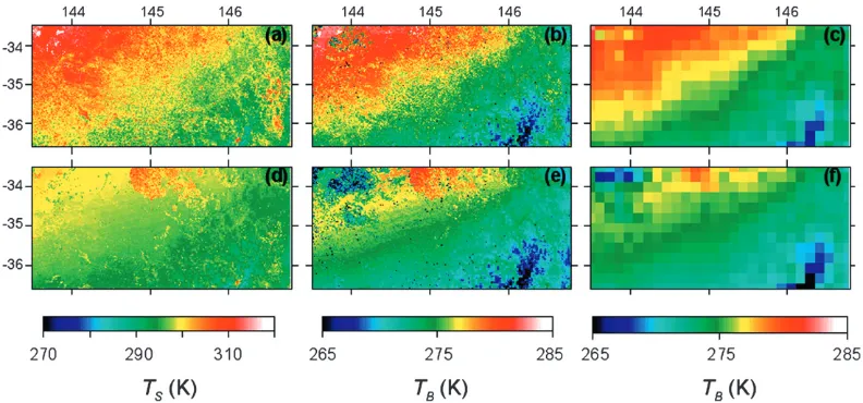
The most common way of estimating land surface temperature from satellite brightness temperature ob-servations is via a split-window algorithm (SWA; Yu et al. 2008). LST retrievals via SWAs (e.g., Becker and Li 1990; Sobrino et al. 1994; Wan and Dozier 1996) exploit the differential absorption of radiation by atmospheric water FIG. 1. Spatial fields of (a) elevation (m) based on the Australian National University DEM (ANUDEM), and (b)
derived 250-m canopy LAI (m2m22). (c) Observed 1-km land surface temperature (K) fromNOAA-18AVHRR sensor thermal bands. (d) Observed 25-km 6.9-GHz brightness temperature (K) fromAquaAMSR-E sensor. Sat-ellite imagery acquired for 2 Oct 2005. Polygon boundary shows the Murrumbidgee River catchment of southeast Australia.
vapor in spectral bands centered approximately on 11 and 12 mm, respectively. They are simple in form
(repre-senting linearizations of the thermal infrared radiative transfer equation) and are thus easy to implement op-erationally for large-scale estimation of LST.
SWA performance is essentially governed by the way in which the algorithm handles atmospheric water con-centration, satellite view angle, and surface emissivity effects. Atmospheric water vapor may be estimated from brightness temperature data themselves (Sobrino et al. 1994), or it may be based on climatologies derived from other satellites or surface observations (Pinheiro et al. 2007). Adjustment for the increase in pathlength with off-nadir observations may be achieved explicitly by varying algorithm coefficients as a function of view angle (Wan and Dozier 1996) or by adding path cor-rection terms to the SWA (Sun and Pinker 2005). The independent estimation of land surface emissivity can be achieved by relatively simple normalized difference veg-etation index–based approaches (Sobrino and Raissouni 2000; Momemi and Saradjian 2007) or by iterative, computational intensive approaches (Gillespie et al. 1998). The resultant accuracy of LST from these methods ranges from 0.4 to 1.75 K (Sobrino et al. 1994; Wan and Dozier 1996; Qin et al. 2001; So`ria and Sobrino 2007; Wan 2008).
In this work, we have used a vegetation classification– based approach to estimate surface emissivity and ap-plied the SWA of Key et al. (1997) to the 11- and 12-mm
channel brightness temperature data from the Advanced Very High Resolution Radiometer (AVHRR) onboard theNational Oceanic and Atmospheric Administration-18
(NOAA-18) polar orbiting satellite. These data have an approximate overpass time for the study area of 1400 LT. All NOAA-18 AVHRR imagery for the period September–November 2005 were obtained from Com-monwealth Scientific and Industrial Research Organisa-tion (CSIRO) archives (King 2003). The SWA coefficients were derived for a range of atmospheric water content and view angle scenarios with the reported accuracy compared with in situ measured LST of,2 K.
Estimates of LST at 1-km resolution across the study area for the relatively cloud-free image on 2 October 2005 are presented in Fig. 1c. Evident in these data is the northwest–southeast gradient in Ts, with higher values
associated with lower LAI in the northwest, whereas coolerTsoccur at higher elevations in mountains and
forests. The fine texture variation inTsshows some
co-incidence with LAI, but it is mediated by soil water availability via the effect of latent and sensible heat loss on canopy temperatures. Water bodies, snow, and small amounts of residual cloud are visible as a speckling of coolerTsacross the region.
3) MICROWAVE BRIGHTNESS TEMPERATURES
The earth’s atmosphere is essentially transparent to microwave radiation in the frequency range 1–15 GHz. Therefore, unlike thermal brightness temperature ob-servations, satellite-based microwaveTbmeasurements
may be considered direct observations of emissions from the land surface. The accuracy of microwave brightness temperature measurements is therefore a function of antenna characteristics and signal deconvolution strat-egies (Ashcroft and Wentz 2000). Reported instrument errors for Tb from the Scanning Multichannel Micro-wave Radiometer (SMMR) onboard Nimbus are be-tween 0.3 and 0.7 K (Njoku and Li 1999). Brown et al. (2008) claim that antenna error contributes 0.9 K to the overall radiometric accuracy of 1.68 K for the Microwave Imaging Radiometer with Aperture Synthe-sis (MIRAS) onboard the planned Soil Moisture and Ocean Salinity (SMOS) satellite (Barre´ et al. 2008). Similarly, the planned Soil Moisture Active Passive (SMAP) instrument has specification for a brightness temperature relative accuracy of 1.5 K (available online at http://smap.jpl.nasa.gov). Another factor affecting the microwave brightness temperature accuracy in un-guarded frequency bands (e.g., those centered on 6.9 and 10 GHz) is radio frequency interference (RFI). It has been shown that RFI is likely to contaminate microwave signals in the more populous region of the globe (Njoku et al. 2005). In the Murrumbidgee catchment study area, the error introduced by RFI is likely to be negligible based on the global distribution determined by Njoku et al. (2005), therefore this error is ignored here.
In this work, we have used the microwave brightness temperature observations from the Advanced Micro-wave Scanning Radiometer for Earth Observing System (AMSR-E) aboard theAquasatellite (Njoku et al. 2003) with an approximate overpass time for the ROI of 1330 h (local time). Specifically, we have used the grid-ded level-3 land surface product resampled to a glo-bal 25-km grid [AMSR-E Aqua daily L3 surface soil moisture, interpretive parameters, and quality control Equal-Area Scalable Earth Grids (EASE-Grids; AE_ Land3), available online at http://nsidc.org/] for the pe-riod September–November 2005.
The microwave brightness temperature observation (Tb) from AMSR-E for October 2005 (Fig. 1d) shows a
different spatial pattern toTsacross the study area. The
two regions whereTbare highest (;280 K) occur in the
northwest–southeast across the ROI. Three areas of coolest Tb are marked A1–A3 in Fig. 1d and are dis-cussed further in section 4.
4. Results
a. Modeled Tsand Tb
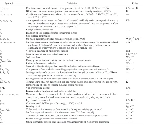
Observation operatorsHtandHmwere used to com-pute modeledTs and Tb, respectively, across the study area for daily modeled soil moisture between 1 Sepber 2005–1 NovemSepber 2005 (see later discussion of tem-poral variation in proportional constraint) and for two extremes of soil moisture content (i.e., wilting point and field capacity) on 2 October 2005. The single model output provides a spatial estimate of the variability in upper and lower bounds ofTs and Tb across the ROI (Fig. 2) corresponding to wilting point and field capac-ity modeled temperatures, respectively. Comparison of Fig. 1c with Figs. 2a and 2d show that observedTsfrom the
AVHRR on this day are bounded by the upper and lower modeled values ofTs, except for pixels contaminated by
water, snow, or cloud. Thus, soil moistures for each pixel in Fig. 1c reside within the range between wilting point and field capacity for this region. It can also be seen that the range in modeled Ts (difference between top and bottom panels) is greatest in the lowest relief and lowest LAI parts of the landscape, whereas the least range inTs occurred in the mountain forests of the southeast.
Modeled Tb (Figs. 2b and 2e) shows a similar southwest–northeast banding as Ts across the ROI.
Aggregation of the 1-km grid cells to 25 km (Figs. 2c and 2f) allowed for direct comparison with observedTb (Fig. 1d). Once again, the observedTbis bounded by the upper and lower modeledTb(Figs. 2c and 2f),
ex-cept for areas marked A1–A3 in Fig. 1d. These areas have lowerTbthan estimated by the model even at field
capacity, suggesting that either standing water is pre-sent on the soil surface at the time of image acquisition or that open water in dams or lakes is ‘‘contaminating’’ observedTb. Although major dams and lakes are as-sociated with these areas (A1 is centered on Hume Dam, A2 is on the hydroelectric water supply dams of Lakes Eucumbene and Jindabyne, and A3 is on the natural intermittently filled Lake George), there is also temporal variation inTbfor these areas between Sep-tember and November 2005 (data not presented). This indicates that intermittent standing water is a key fac-tor that is likely to influence microwave emissions from these areas.
The range inTbis greatest in the northwest where a
large fraction of bare soil is visible to the sensor. The range in Tb is least for the high relief, tall forests
(marked A2 in Fig. 1d) as a result of the presence of the high biomass, strong relief, and high vegetation moisture contents, which act to scatter passive microwave emis-sions from the soil. In addition, as explained earlier, the differences in the pixel pattern of modeled and observed Tbin area A2 is due to dams of the Snowy Mountains
Hydroelectric Scheme’s remaining snowpack at the highest elevations and surface water, which interferes with the soil passive microwave signal.
FIG. 2. Spatial fields for the Murrumbidgee River catchment region of southeastern Australia of (a),(d) modeled 1-km thermal land surface temperature (K) derived from the observation operatorHt. (b),(e) Modeled 1-km mi-crowave land surface brightness temperature (K) derived from the observation operatorHm. (c),(f) Microwave brightness temperature (K) from (b) and (e) aggregated to 25 km. Shown is the output for (top) minimum (wilting point) and (bottom) maximum (field capacity) soil moisture contents.
The range of modeledTsin Figs. 2a and 2d is plotted
as a function of LAI for the three vegetation types in Figs. 3a and 3c. The highest surface temperatures for soils at wilting point (Fig. 3a) are associated with an increasing fraction of bare soil (LAI,2). At field ca-pacity (Fig. 3c), higher rates of evapotranspiration from soil and vegetation suppressed the range in modeledTs
across all LAI, with the most pronounced effects when LAI was less than 2.
Similar analyses were conducted on modeled micro-wave brightness temperature (Fig. 4). The range of modeledTbin Figs. 2b and 2c is plotted as a function of
LAI in Figs. 4a and 4c. These data show an increase in
Tbwith decreasing LAI in dry soils. This increase inTb
(Fig. 4a) is due to both a decrease in the surface di-electric constant under dry conditions at lower biomass densities and a higher soil source temperature with
in-creased radiation incident on the soil surface. For soils at field capacity (Fig. 4c), modeled Tb was up to 5 K
lower than at wilting point for pixels where LAI was,2. At these LAI, the microwave emissions from the soil surface dominated the Tbsignal over vegetation
mois-ture. At higher LAI, the soil signal was progressively at-tenuated by biomass microwave emissions, and the difference betweenTbat wilting point and field capacity
approached zero.
b. Model sensitivity
Sensitivity of modeledTsto perturbations in the two
extremes of soil moisture status (dTs/duz) were
com-puted and displayed as functions of LAI in Figs. 3b and 3d. The sensitivity is greater (more negative) under dry soils (Fig. 3b) than at field capacity (Fig. 3d), partic-ularly when LAI was.2. However, sensitivities differed
FIG. 3. Scatterplots of (a),(c) modeled land surface temperature (K) derived from the observation operatorHt
and (b),(d) sensitivity of land surface temperature to profile average soil moisture content (dTs/du
z) from the tangent linear model ofH t
between the three vegetation classes. Relatively low sensitivities were observed for shrublands at all LAI and for all vegetation classes when LAI approached zero. Maximal sensitivity was observed for forests and grass-lands/crops at high LAI (Fig. 3b). The sensitivity was suppressed in forest and grassland/crops when soils were at field capacity (Fig. 3d). Differences in sensitivities among vegetation types are due to physiological differ-ences in maximum stomatal conductance to water vapor (gmax) between these classes (gmaxforest, 10 mm s21; grassland/crop, 20 mm s21
; shrub55 mm s21
;) based on Jones 1992 and Bell and Williams 1997. The banding of points evident within a vegetation class (e.g., Fig. 3b) arose from soils of different soil moisture holding ca-pacities (umax2umin). Higher sensitivity was observed for soils having lower water holding capacity.
Modeled brightness temperature sensitivity (dTb/dus1) under dry soils is highest (most negative) for LAI,2.5
(Fig. 4b), but it rapidly diminishes to zero at LAI.3 as a result of vegetation microwave emissions obscuring the soil signal. For soils at field capacity, the sensitivity remains strong even at relatively high LAI (i.e., between 25 and210 up to an LAI’4) with differences in sen-sitivity evident among vegetation classes (e.g., shrub-lands are more sensitive than grassland/crops).
c. Analysis error
The relationship between model sensitivity to per-turbation in soil moisture (dT/du) and analysis, obser-vation, and background variances (sa,so, and sb) are illustrated for the scalar case [Eq. (3)] in Fig. 5 for ‘‘ac-curate’’ and ‘‘uncertain’’ modeled soil moistures. Note that this analysis assumes that the model bias in soil moisture (propagated through the observation opera-tors to bias in modeledTsorTb) and observation bias
has been already eliminated. In each case, the rate at FIG. 4. Scatterplots of (a),(c) modeled microwave brightness temperature (K) derived from the
obser-vation operatorHm
and (b),(d) sensitivity of brightness temperature to surface layer soil moisture content (2.5-cm depth;dTb/dus1) from the tangent linear model ofHm
as a function of LAI. Plots show model output for (a),(b) wilting point and (c),(d) field capacity soil moisture contents. Points derived as in Fig. 3. Black, gray, and white symbols refer to forest, shrub, and grassland/crop vegetation classes, respectively.
which the analysis error (sa) approached the back-ground error (sb) varied depending on the sensitivity termdT/du: the lower the sensitivity (less negative), the more rapidly sa approached sb and the poorer the constraint provided by an observation. The rate at which these curves approached the limitsbalso depended on sb itself. In Table 1, we considered the proportional constraint [Eq. (4)] as a measure of efficacy of the ob-servations to constrain modeled soil moisture in the as-similation for three cases of observation error, two background errors (sb50.025 m3m23
and 0.05 m3m23
), and three sensitivities (dT/du 5 22.5,210, and225). The three cases of observation error (so51.25, 0.5, and 0.25 K) were chosen based on published errors (from section 3c).
At low sensitivities (dT/du5 22.5), an observation of error 51.25 K provided virtually no constraint on the model. In this case, the proportional constraint [Eq. (4)] was ,1%. However, when sensitivities were greater (dT/du 5 210), a reduction in error of up to 7% was observed with an observation error of 1.25 K. With an increase in the observation accuracy to 0.5 K, the rela-tive constraint increased to.10% for the accurate case but up to;30% for the uncertain case. At higher sen-sitivities, such as those observed for microwaveTb(Figs. 4b and 4d), the proportional constraint provided byso5 1.25 K is substantial (29%) when the background soil moisture was ‘‘uncertain’’ and increased considerably to
;63% for observation errors of 0.5 K. Further
im-provements in the observation error to within the noise of the instrument (so50.25 K) yielded significant im-provements in the reduction of analysis error (Table 1) but observations of this accuracy from satellite are un-likely in the foreseeable future.
Temporal variation in the proportional constraint [Eq. (4)] provided byTsandTbobservations is shown in Figs. 6a, 6b, 7a, and 7b for two contrasting vegetation types: semiarid woodlands and tall forests. In semiarid open woodlands and under moist conditions following rainfall, the reduction in background error inus1afforded byTbobservations can be up to 50% or 30% for
uncer-tain and accurate cases, respectively (Fig. 6a). However, this constraint reduces rapidly to zero as soils dry. In contrast,Tsobservations provide virtually no reduction
in background error inuzfor open woodlands (Fig. 6b). For tall forests, the reduction in background error inus1 from the assimilation ofTbobservations (Fig. 7a) was an order of magnitude less than for semiarid woodlands (Fig. 7a) but with the same decrease in proportional constraint as the soil surface dried (Fig. 7a). The reduc-tion in background error provided by Ts observations was up to 8% for the uncertain case (Fig. 7b); however, in this case the constraint onuzincreased as the soil profile dried rather than decreased as for Tb. For a cropping/ pasture site in the central Murrumbidgee catchment, the proportional constrain provided byTsandTb
observa-tions was midway between these extremes, with each observation type contributing up to a maximum of 10% and 20%, respectively (data not presented).
The bottom panels of Figs. 6c and 7c provide pre-liminary information on model-observation bias. In the semiarid woodland, modeled Ts consistently under-estimated observations by an average of 4.0 K and modeled Tb consistently overestimated observations, particularly when rainfall was frequent and/or heavy, by an average of 9.6 K (Fig. 6c). For tall forests (Fig. 7c), these model-observation biasesTsandTbwere reduced to an average of 1.6 and 1.8 K, respectively, but with the TABLE1. Proportional constraint (sb2sa/sb) for observations
of given error (so) as quantified by Eq. (4), given three sensitivities
of observed temperature against perturbation in soil moisture content [dT/du; K (m3m23)21] and two background errors [s
b5
0.025 m3m23(accurate case) and 0.05 m3m23(uncertain case)].
sb dT/du
so(K)
(m3m23) [K (m3m23)21] 0.25 (%) 0.5 (%) 1.25 (%)
0.025 22.5 3.0 0.8 0.1
210 29.3 10.6 1.9
225 62.9 37.5 10.6
0.05 22.5 10.6 3.0 0.5
210 55.3 29.3 7.2
220 80.4 62.9 29.3
FIG. 5. Effect of observation error (so) on error in analysis state
variables (sa). The various curves correspond to different
sensi-tivities of temperature to soil moisture contents (dT/du) ranging from21 to225 K m3m23. Two sets of curves are shown: black
curves correspond to a background standard deviation (sb) of
0.025 m3m23
same sign. This result indicates a better performance by the water balance model in tall forests rather than in semiarid woodlands but with potentially similar sources of bias.
5. Discussion
The efficacy of an observation type as a constraint on hydrological and hydrometeorological models is a function of the sensitivity of modeled observation to perturbation in the model state, the observation error, and the background error, and is expressed as the dif-ference (relative or absolute) between the analysis and background errors. This study has shown that both thermal and microwave satellite observations can pro-vide effective observational constraint on the modeled profile and surface soil moisture contents but only under certain conditions. Furthermore, the characteristics at which the observational constraint is maximal forTsand
Tbobservations are complimentary—a fact that can be
exploited to improve the estimation of soil moisture by satellite observations. Under a weak constraint, the water balance model will operate through time without any feedback from observations. However, under con-ditions where thermal and microwave observations to-gether or separately provide a strong constraint, the model is benefited by a sequential adjustment that takes
into consideration the orthogonal information con-tained in each observation type.
The fact that the observedTbandTs(Figs. 1c and 1d) fall within the endpoints of modeledTbandTs(Fig. 2)
confirms that the observation operatorsHtandHmare
functioning realistically in this study, given available climate, soils, and vegetation data. The exception is where errors were introduced by standing water, snow, and cloud, as these conditions are not represented by the observation operators (these would be masked out in an operational assimilation scheme). The analysis of model sensitivities to perturbation in states showed that the sensitivity ofTsto profile moisture content was minimal in circumstances where low maximal stomatal conduc-tance is an inherent plant trait (e.g., in shrublands), large fractions of soil surface were visible to the sensor (i.e., low LAI), soil water holding capacity was large (i.e., largeumax2umin), and/or profile soil moisture content
was near saturation (Fig. 3). Conversely, the sensitivity
ofTbto surface layer soil moisture was minimal under
conditions of high LAI, dense woody biomass, and low soil moisture content (Fig. 4). Maximal sensitivity forTs occurred under drying soil —where vegetation stomata were strongly responsive to available water, such as in sands and sandy-loam soils, which have a smaller wa-ter holding capacity than clay soils—and at high LAI (Fig. 3). These results highlight the importance of FIG. 6. Temporal sequence of (a) the proportional constraint [Eq. (4); left axis] provided by
microwaveTb(so50.5 K; dashed line,sb50.025 m3m23; and dotted line,s
b50.05 m3m23) and surface layer volumetric moisture content (solid line; right axis). (b) Proportional con-straint (left axis) provided byTs(so50.75 K; dashed line,sb50.025 m3m23; dotted line,s
b5 0.05 m3m23) and profile soil moisture content (solid line; right axis). (c) Modeled and observed Ts(dashed line and closed symbols; left axis),Tb(solid line and open symbols; left axis) and rainfall (bars; right axis) for a grid cell/pixel in the western Murrumbidgee catchment. Location was a semiarid open woodland/shrubland (LAI51.3 andgmax55 mm s21).
accurate information on soil and vegetation physical properties because dT
s/duz is dependent on both the
range in soil moisture between wilting point and field capacity and canopy cover. Under conditions of maxi-mal sensitivity, maximum information on soil moisture content from an observation is mapped to state variables by the assimilation. In the ROI, this occurred primarily throughout the moderate-to-high relief and in well-developed canopies of the forest, cropping regions, and pastures (LAI.2) in a band that extended from the northeast to south and southeast in Fig. 1. Little infor-mation on profile soil moisture content was provided by Tsobservations under sparse canopies in the flat terrain
of the western part of this ROI (Fig. 3).
The conditions under whichTsandTbprovide strong
constraints onuzandus1are approximately the converse
for each observation type (Figs. 6 and 7). This means that the prospect for significant improvements in model performance by employing both observation types at the same time within a data assimilation scheme is consid-erable. This is because when conditions vary such that one observation type is ineffective at constraining model soil moisture, the other observation type can potentially act as a strong constraint on model dynamics. This dy-namic variation in the proportional constraint is evi-denced in Figs. 6a, 6b, 7a, and 7b where an initially wet profile undergoes drying to near-wilting point, with more rapid drying of the surface layers than deeper in the profile. In a wet soil and full canopy with stomata fully open, observations ofTsprovide little constraint on
profile moisture content (Fig. 7b), whereas microwave observations of Tb provide a stronger constraint on
surface layer moisture (Fig. 7a). With the drying of the upper soil layers, observations ofTbcease to constrain
modeled surface moisture content, whereas observa-tions ofTsprovide an increasingly strong constraint on
profile moisture content. For a semiarid location, the majority of the observational constraint through time was provided by microwave observations of surface soil moisture, particularly under wet soils (Fig. 6a) with little constraint on u
z provided by observations ofTs. This
dynamic variation in the strength of observational con-straints from multiple satellite sensors can be exploited in regional-scale hydrological and hydrometeorologi-cal data assimilations using ‘‘multiple constraints’’ ap-proaches (e.g., Barrett 2002; Barrett et al. 2005; Raupach et al. 2005; McCabe et al. 2008; Renzullo et al. 2008) that also take into account the varying frequency of observa-tions (Figs. 6c and 7c) to provide the most accurate esti-mation of soil moisture initial conditions possible. This will lead to subsequent benefits for the prediction of la-tent and sensible heat fluxes to the atmosphere, runoff, streamflow, and soil water availability.
The magnitude of observation errors is critical in de-termining the efficacy of satellite data as constraints on models. Increasing measurement error, bias, and infre-quent data reduce the effectiveness of observations as constraints (Figs. 5–7; Table 1). Currently, the range in accuracy for observedTsfrom SWAs is 0.4–1.75 K (see
section 2c), and the present study has shown that for
so.1.5 K, these errors are too large for satellite thermal
observations to be an effective constraint on modeled soil moisture content, especially when the background error is small (e.g., sb 5 0.025 m3 m23
in Fig. 5). For an FIG. 7. Same as Fig. 6 but for a grid cell/pixel in the eastern Murrumbidgee catchment located in
uncertain background (0.05 m3m23), these observations provide a marginal improvement in the analysis errors but only under conditions when the sensitivity (dTs/du
z)
is maximal. It would appear, therefore, that the prospects for individual thermal observations imparting constraint on profile soil moisture estimation will only improve if observation error can be reduced to;1 K. Despite the apparent limitation this may impose, the serial nature of satellite observations, their spatial and temporal corre-lations, and the ‘‘memory’’ of soil moisture stores con-tained in the model equations act to stabilize model dynamics in a time series when observations have large errors or are absent. Further work is needed to deter-mine how to best exploit multiple thermal observations acquired at key times of the day (Kustas and Norman 1999; Anderson et al. 2007; Crow et al. 2008) and to in-corporate vegetation greenness (Gillies and Carlson 1995; Carlson 2007) to further improve estimates of root-zone soil moisture.
In the case of microwaveTb, the requirement for close
tolerances on observation errors is to some degree ob-viated by the strong sensitivity (Fig. 4), and any im-provement in the accuracy of these observations would be expected to further increase the strong constraint on modeledus1(Fig. 5). These results concur with estimated
error reduction using ensemble Kalman filter methods by Reichle et al. (2002). They found a reduction in root-mean-square error for surface soil moisture of up to
;80% using passive microwave when compared against values obtained without assimilation. However, these improvements can only be achieved where the potential bias from an incorrect specification of canopy optical depth, soil temperature, surface roughness, and surface emissivity is removed—and these biases can be sub-stantial (Draper et al. 2009; Wagner et al. 2007). As-suming that these biases can be eliminated through the accurate and independent estimation of LAI and optical depth, the use of a coupled SEB–MRT model to provide soil and vegetation temperatures, and through accurate information on soil physical properties, the prospects for improved prediction of surface soil moisture from data assimilation constrained by passive microwave obser-vations is good. The exceptions to this are the conditions under which the sensitivity ofTbis low or where the
observation operator performs badly, such as in moun-tainous terrain, high biomass forests, or where standing water or snow is present.
Comparison of modeled observations with satellite data (Figs. 6c and 7c) showed the consistent underestimation of
Tsand overestimation ofTbby the water budget but with
less bias evident for the tall forest site (Fig. 7c) than for open woodland (Fig. 6c). The identification of biases through the application of multiple constraints data
as-similation is one of the major benefits of these methods. The sharp reduction inTbfollowing rainfall relative to the
model (Fig. 6c) is strongly suggestive of surface saturation and possibly pooling of water in run-on parts of the landscape. Consistent underestimation ofTsis indicative
of a modeled profile that is too wet relative to observa-tions, which may indicate the possible underestimation of drainage or evapotranspiration terms of the model. Fur-ther work is required to elucidate the nature of these biases, to determine whether they arise from observations or from the model, to determine their spatial and tem-poral variations, and to develop correction functions for use in an operational data assimilation scheme.
6. Conclusions
The tangent linear model (TLM) for two observation operators were used to examine the sensitivities of thermal and microwave satellite observations to varia-tions in profile and surface layer soil moisture. The TLM forTsshowed the strongest sensitivity when soils were
relatively dry, in grassland/crop and forest vegetation classes, at low soil water holding capacity, and when canopy leaf area index (LAI) exceeded 2.5. Low sensi-tivity ofTswas observed where soils were at field
ca-pacity (across all vegetation types), in shrublands (as a result of low maximum stomatal conductance), and in sparse canopies where bare soils prevailed. The TLM for
Tbshowed sensitivities 1–10 times greater than forTs.
Maximal sensitivities of Tb to surface soil moisture
content occurred when LAI was,1.5 in dry soils but up to an LAI of;4 when soils were at field capacity.
Satellite observations of thermal and microwave emissions of the land surface can provide strong straints on root-zone soil moisture under specific con-ditions. Where potential sources of bias are eliminated and the observation errors reduced to;1 K, these ob-servations offer good prospects for improved profile soil moisture prediction—particularly when combined in a ‘‘multiple constraints’’ data assimilation context. The multiple constraints methods have additional benefits of using orthogonal information in observations to in-crease the observational constraint on model dynamics and in identifying the presence of bias in the model and/ or observations.
Acknowledgments.The authors acknowledge support and funding for this work from the CSIRO Land and Water ‘‘Innovation Bank’’ and from the CSIRO Water for a Healthy Country Flagship Program. Constructive and helpful suggestions were also provided by Dr. Ray Leuning of CSIRO Marine and Atmospheric Research and three anonymous referees.
APPENDIX
Observation Model Operators and TLM Approximations
Observation model operators and their respective TLM representation are given here. The observation
operator for land surface temperatureHtwas developed
from the equations of Friedl (1995, 2002) using the Jarvis (1976) formulation for canopy resistance to water va-por and the stomatal resistance scaling functions of Cox et al. (1998). The observation operator for
micro-wave brightness temperatureHmwas based on the
mi-crowave radiative transfer theory presented in Wang and Schmugge (1980), Mo et al. (1982), Dobson et al. (1985), Njoku et al. (2003), and Owe et al. (2001).
(For more details, including model assumptions and limitations, refer to the references above.) Here only the pertinent components of each model for
calcu-lating temperature (Ts or Tb) and the TLM are
pre-sented. Model variables and parameters are defined in Table A1.
a. Land surface temperature
The SEB model used in this work comprised six non-linear equations that describe the portioning of moisture and heat fluxes between the vegetation and soil surface layers and the overlying atmosphere (Friedl 2002). Key
TLM equations are denoted by a d symbol preceding
each variable. Active variable in case of LST isuz. A
simple N-loop construct was considered the most
effi-cient method of numerically solving the equations for
TABLEA1. Symbols used in tangent linear model equations of the appendix.
Symbol Definition Units
c1,c2,c4 Constants used to scale water vapor pressure function; 0.611, 17.22, and 35.86 kPa, — , K
c3 Offset used in water vapor pressure and microwave emissivity functions; 273.15 K
c5,c6,c7,c8 Coefficient used to calculate dielectric constant of water; 88.045,20.4147, 6.29531024,
and 1.07531025 —
ea,e0,ey*,ess Atmospheric vapor pressure of the mixed layer (a) and height of exchange within canopy (0); saturated water vapor pressure at leaf temperature (y); and vapor pressure of air in soil spaces between 0 and 2.5-cm depth (ss)
kPa
er Rough surface emissivity —
fss Fraction of soil surface visible to thermal sensor —
h Soil surface roughness —
p2,p3,p4 Stomatal resistance model parameters (Cox et al. 1998) W m22, kPa21,–
ra,rb,rw,ry,rss Surface aerodynamic resistance to water vapor and heat exchange (a); resistance to heat exchange by foliage (b) and soil surface soil surface (w); and resistance to the exchange of water vapor by canopy (y) and soil surface (ss)
s m21
Au View zenith angle of microwave sensor rad
Cp Specific heat of air at constant pressure J kg21K21
G Soil heat flux W m22
Gmax,Gmin Canopy maximum and minimum conductance to water vapor m s21
Isw Incident shortwave radiation W m22
R Smooth soil reflectivity to horizontally polarized microwave radiation —
Rny, Rns Component of net radiation reaching vegetation canopy (yand soil surface (s) W m22
Sl,Sy,Su Scaling function of stomatal conductance for incoming shortwave radiation (l), VPD (y),
and average profile soil moisture content (u)
—
Su
s1 Scaling function of stomatal conductance for soil moisture from 0 to 2.5-cm depth —
T0,Ty,Tss Temperature of air at height of heat and water vapor exchange within the canopy (0), temperature of canopy foliage (y), and soil surface (ss)
K
VPD Vapor pressure deficit kPa
b Linear scaling function of soil water availability —
«,«a,«i,«r,«w,«x Microwave dielectric constant of soil, water, and air mixture; dielectric constant of air (a), ice (i), rock (r), and water (w); and water absorbed by clay (x) in the soil
—
g Psychometric constant kPa K21
gWS Constant used in Wang and Schmugge (1980) model —
r Density of air kg m23
umax,umin Volumetric soil moisture at field capacity (max) and wilting point (min) m3m23
us1 Surface layer volumetric soil moisture content (0–2.5-cm depth) m3m23
ut ‘‘Transition’’ soil moisture content where soil moisture saturates pore spaces m3m23
uz Profile average volumetric soil moisture content m3m23
the temperatures and water vapor pressure values and computing the TLM. The method was found to rapidly converge to solution (e.g., temperature estimates con-verged to within 0.5 K withinN55 iterations). Com-putation begins with the initializationTy5T05Tss5
Ts5fssTss1(1 fs)Ty
dTs5fssdTss1(1 fss)dTy.
} Algorithm End.
b. Microwave brightness temperature
The coupled SEB–MRT model used in this work uses the soil and vegetation temperatures computed in the SEB model earlier. Key TLM equations are denoted by
adsymbol preceding each variable. Active variable in
case of microwave brightness temperature isus1. Again,
a simpleN-loop construct was considered the most
d«5(« J. R. Mecikalski, 1997: A two-source time-integrated model for estimating surface fluxes using thermal infrared remote sensing.Remote Sens. Environ.,60,195–216.
——, ——, J. R. Mecikalski, J. A. Otkin, and W. P. Kustas, 2007: A climatological study of evapotranspiration and moisture stress across the continental United States based on thermal remote sensing: 1. Model formulation.J. Geophys. Res.,112,D10117, doi:10.1029/2006JD007506.
Ashcroft, P., and F. J. Wentz, 2000: AMSR level 2A algorithm. Algorithm theoretical basis document, Remote Sensing Sys-tems Tech. Rep. 121599B-1, 29 pp.
Aubert, D., C. Loumange, L. Oudin, and S. Le Hegarat-Mascale, 2003: Assimilation of soil moisture into hydrological models: The sequential method.Can. J. Remote Sens.,29, 711–717.
Australian Survey and Land Information Group, 1990:Vegetation. Vol. 6,Atlas of Australian Resources,Third Series, Depart-ment of Administrative Services, Commonwealth of Australia, 64 pp. [Available online at http://www.ga.gov.au/image_cache/ GA10358.pdf.]
Bach, H., and W. Mauser, 2003: Methods and examples for remote sensing data assimilation in land surface process modelling. IEEE Trans. Geosci. Remote Sens.,41,1629–1637.
Barre´, H. M. J. P., B. Duesmann, and Y. Kerr, 2008: SMOS: The mission and the system.IEEE Trans. Geosci. Remote Sens.,46, 587–593.
Barrett, D. J., 2002: Steady state turnover time of carbon in the Australian terrestrial biosphere.Global Biogeochem. Cycles, 16,1108, doi:10.1029/2002GB001860.
——, M. J. Hill, L. B. Hutley, J. Beringer, J. H. Xu, G. D. Cook, J. O. Carter, and R. J. Williams, 2005: Prospects for improved
savanna biophysical models by using multiple-constraints model-data assimilation methods.Aust. J. Bot.,53,689–714. ——, V. A. Kuzmin, J. P. Walker, T. R. McVicar, and C. Draper,
2008: Improving stream flow forecasting by integrating satel-lite observations, in situdata and catchment models using model-data assimilation methods. eWater Cooperative Re-search Centre Tech. Rep., 54 pp. [Available online at http:// ewatercrc.com.au/reports/Barrett_et_al-2008-Flow_Forecasting. pdf.]
Becker, F., and Z.-L. Li, 1990: Towards a local split window method over land surfaces.Int. J. Remote Sens.,11,369–393. Bell, D. T., and J. E. Williams, 1997: Eucalypt physiology.
Eu-calypt Ecology: Individuals to Ecosystems,J. E. Williams and J. C. Z. Woinarski, Eds., Cambridge University Press, 168–196.
Boni, G., D. Entekhabi, and F. Castelli, 2001: Land data assimila-tion with satellite measurements for the estimaassimila-tion of surface energy balance components and surface control on evapora-tion.Water Resour. Res.,37,1713–1722.
Boussetta, S., T. Koike, K. Yang, T. Graf, and M. Pathmathevan, 2008: Development of a coupled land–atmosphere satellite data assimilation system for improved local atmospheric simulations.Remote Sens. Environ.,112,720–734.
Bouttier, F., and P. Courtier, 1999: Data assimilation concepts and methods. Meteorological Training Course Lecture Notes, ECMWF, 58 pp.
Brown, M. A., F. Torres, I. Corbella, and A. Colliander, 2008: SMOS Calibration.IEEE Trans. Geosci. Remote Sens.,46, 646–658.
Cai, W. J., and T. Cowan, 2008: Evidence of impacts from rising temperature on inflows to the Murray-Darling Basin. Geo-phys. Res. Lett.,35,L07701, doi:10.1029/2008GL033390. Caparrini, F., F. Castelli, and D. Entekhabi, 2004: Estimation of
surface turbulent fluxes through assimilation of radiometric surface temperature sequences.J. Hydrometeor.,5,145–159. Carlson, T., 2007: An overview of the ‘‘Triangle Method’’ for
es-timating surface evapotranspiration and soil moisture from satellite imagery.Sensors,7,1612–1629.
Cox, P. M., C. Huntingford, and R. J. Harding, 1998: A canopy conductance and photosynthesis model for use in a GCM land surface scheme.J. Hydrol.,212-213,79–94.
Crosson, W. L., C. A. Laymon, R. Inguva, and M. P. Schamschula, 2002: Assimilating remote sensing data in a surface flux-soil moisture model.Hydrol. Processes,16,1645–1662.
Crow, W. T., M. Drusch, and E. F. Wood, 2001: An observation system simulation experiment for the impact of land surface heterogeneity on AMSR-E soil moisture retrievals. IEEE Trans. Geosci. Remote Sens.,39,1622–1631.
——, W. P. Kustas, and J. H. Prueger, 2008: Monitoring root-zone soil moisture through the assimilation of a thermal remote sensing-based soil moisture proxy into a water balance model. Remote Sens. Environ.,112,1268–1281.
de Jeu, R. A. M., and M. Owe, 2003: Further validation of a new methodology for surface moisture and vegetation optical depth retrieval.Int. J. Remote Sens.,22,4559–4578.
de Lannoy, G. J. M., R. H. Reichle, P. R. Houser, V. R. N. Pauwels, and N. E. C. Verhoest, 2007: Correcting for forecast bias in soil moisture assimilation with the ensemble Kalman filter.Water Resour. Res.,43,W09410, doi:10.1029/2006WR005449. Dobson, M. C., F. T. Ulaby, M. T. Hallikainen, and M. A. El-Rayes,
1985: Microwave dielectric behavior of wet soil-Part II: Di-electric mixing models.IEEE Trans. Geosci. Remote Sens., GE-23,35–46.
Draper, C. S., J. P. Walker, P. J. Steinle, R. A. M. de Jeu, and T. R. H. Holmes, 2009: An evaluation of AMSR-E derived soil moisture over Australia.Remote Sens. Environ.,113,703–710. Entekhabi, D., H. Nakamura, and E. G. Njoku, 1994: Solving the inverse problem for soil moisture and temperature profiles by sequential assimilation of multifrequency remotely sensed observations.IEEE Trans. Geosci. Remote Sens.,32,438–448. Errico, R. M., 1997: What is an adjoint model?Bull. Amer. Meteor.
Soc.,78,2577–2591.
Friedl, M. A., 1995: Modeling land surface fluxes using sparse canopy model and radiometric surface temperature mea-surements.J. Geophys. Res.,100(D12), 25 435–25 466. ——, 2002: Forward and inverse modeling of land surface energy
balance using surface temperature measurements. Remote Sens. Environ.,79,344–354.
Gao, H., E. F. Wood, T. J. Jackson, M. Drusch, and R. Bindlish, 2006: Using TRMM/TMI to retrieve surface soil moisture over the southern United States from 1998–2002.J. Hydrometeor.,
7,23–38.
Giering, R., 2000: Tangent linear and adjoint biogeochemical models. Inverse Methods in Global Biogeochemical Cycles, Geophys. Monogr.,Vol. 114, Amer. Geophys. Union, 33–48. ——, and T. Kaminski, 1998: Recipes for adjoint code construction.
ACM Trans. Math. Software,24,437–474.
Gillespie, A., S. Rokugawa, T. Matsuna, J. S. Cothern, S. Hook, and A. B. Kahle, 1998: A temperature and emissivity separa-tion algorithm for advanced spaceborne thermal emission and reflection radiometer (ASTER) images.IEEE Trans. Geosci. Remote Sens.,36,1113–1126.
Gillies, R. R., and T. N. Carlson, 1995: Thermal remote sensing of surface soil water content with partial vegetation cover for incorporation into climate models.J. Appl. Meteor.,34, 745–756.
Heathman, G. C., P. J. Starks, L. R. Ahuja, and T. J. Jackson, 2003: Assimilation of surface soil moisture to estimate profile soil water content.J. Hydrol.,279,1–17.
Hill, M. J., U. Senarath, A. Lee, M. Zeppel, J. M. Nightingale, R. J. Williams, and T. R. McVicar, 2006: Assessment of the MODIS LAI product for Australian ecosystems.Remote Sens. Environ.,101,495–518.
Huang, C., X. Li, and L. Lu, 2008: Retrieving soil temperature profile by assimilating MODIS LST products with ensemble Kalman filter.Remote Sens. Environ.,112,1320–1336. Jackson, R. B., J. Canadell, J. R. Ehleringer, H. A. Mooney,
O. E. Sala, and E. D. Schulze, 1996: A global analysis of root distributions for terrestrial biomes. Oecologia, 108, 389–411.
Jarvis, P. G., 1976: The interpretation of the variations in leaf water potential and stomatal conductance found in canopies in the field.Philos. Trans. Roy. Soc. London,B273,593–610. Jeffrey, S. J., J. O. Carter, K. B. Moodie, and A. R. Beswick, 2001:
Using spatial interpolation to construct a comprehensive ar-chive of Australian climate data.Environ. Modell. Software,
16,309–330.
Jones, A. S., T. Vukicevic, and T. H. Vonder Haar, 2004: A mi-crowave satellite observational operator for variational data assimilation of soil moisture.J. Hydrometeor.,5,213–229. Jones, H. G., 1992:Plants and Microclimate: A Quantitative
Ap-proach to Environmental Plant Physiology. Cambridge Uni-versity Press, 428 pp.
Key, J. R., J. B. Collins, C. Fowler, and R. S. Stone, 1997: High-latitude surface temperature estimates from thermal satellite data.Remote Sens. Environ.,61,302–309.
King, E. A., 2003: The Australian AVHRR data set at CSIRO/ EOC: Origins, processes, holdings and prospects. CSIRO Earth Observation Centre Rep. 2003/04, 51 pp. [Available online at http://www.eoc.csiro.au/tech_reps/2003/tr2003_04.pdf.] Koster, R. D., M. J. Suarez, and M. Heiser, 2000: Variance and
predictability of precipitation at seasonal-to-interannual timescales.J. Hydrometeor.,1,26–46.
Kustas, W. P., and J. M. Norman, 1999: Evaluation of soil and vegetation heat flux predictions using a simple two-source model with radiometric temperatures for partial canopy cover.
Agric. For. Meteor.,94,13–25.
McCabe, M. F., H. Gao, and E. F. Wood, 2005: Evaluation of AMSR-E-derived soil moisture retrievals using ground-based and PSR airborne data during SMEX02.J. Hydrometeor.,6, 864–876.
——, E. F. Wood, R. Wojcik, M. Pan, J. Sheffield, H. Gao, and H. Su, 2008: Hydrological consistency using multi-sensor re-mote sensing data for water and energy cycle studies.Remote Sens. Environ.,112,430–444.
McKenzie, N., and J. Hook, 1992: Interpretation of the Atlas of Australian Soils. Consulting report to the Environmental Resources Information Network (ERIN), CSIRO Division of Soils Tech. Rep. 94/1992, 7 pp.
Mecikalski, J. R., G. R. Diak, M. C. Anderson, and J. M. Norman, 1999: Estimating fluxes on continental scales using remotely sensed data in an atmosphere–land exchange model.J. Appl. Meteor.,38,1352–1369.
Mein, R. G., and C. L. Larson, 1973: Modeling infiltration during steady rain.Water Resour. Res.,9,384–394.
Merlin, O., A. Chehbouni, G. Boulet, and Y. Kerr, 2006: Assimi-lation of disaggregated microwave soil moisture into hydrologic model using coarse-scale meteorological data.J. Hydrometeor.,
7,1308–1322.
Mo, T., B. J. Choudhury, T. J. Schmugge, J. R. Wang, and T. J. Jackson, 1982: A model for the microwave emission from vegetation-covered fields.J. Geophys. Res.,87(C18), 11 229– 11 238.
Momemi, M., and M. R. Saradjian, 2007: Evaluating NDVI-based emissivities of MODIS bands 31 and 32 using emissivities derived by day/night LST algorithm.Remote Sens. Environ.,
106,190–198.
Monteith, J. L., 1965: Evaporation and environment.The State and Movement of Water in Living Organisms,G. E. Fogg, Ed., Proceedings of the Symposium of the Society of Experimental Biology, Vol. 19, Academic Press, 205–234.
Moran, M. S., C. D. Peters-Lidard, J. M. Watts, and S. McElroy, 2004: Estimating soil moisture at the watershed scale with satellite-based radar and land surface models.Can. J. Remote Sens.,30,805–826.
Njoku, E. G., and L. Li, 1999: Retrieval of land surface parameters using passive microwave measurements at 6-18 GHz.IEEE Trans. Geosci. Remote Sens.,37,79–93.
——, T. J. Jackson, V. Lakshmi, T. K. Chan, and S. V. Nghiem, 2003: Soil moisture retrieval from AMSR-E. IEEE Trans. Geosci. Remote Sens.,41,215–229.
——, P. Ashcroft, T. K. Chan, and L. Li, 2005: Global survey and statistics of radio-frequency interference in AMSR-E land observations.IEEE Trans. Geosci. Remote Sens.,43,938–947. Norman, J. M., and Coauthors, 2003: Remote sensing of surface energy fluxes at 101-m pixel resolutions.Water Resour. Res., 39,1221, doi:10.1029/2002WR001775.