Hybrid Modeling and Control of a
Hydroelectric Power Plant
Giancarlo Ferrari-Trecate, Domenico Mignone, Dario Castagnoli, Manfred Morari
Institut f¨
ur Automatik
ETH - Eidgen¨
ossische Technische Hochschule Z¨
urich
CH-8092 Z¨
urich
Tel. + 41 1 632 7626
Fax + 41 1 632 1211
http://control.ethz.ch
{ferrari,mignone,castagnoli,morari}@aut.ee.ethz.ch
Abstract
In this work we present the model of a hydroelectric power plant in the framework of Mixed Logic Dynam-ical (MLD) systems. Each outflow unit exhibits a hy-brid behaviour since flaps, gates and turbines are con-trolled with logical inputs and the outflow dynamics depend on the logical state of the unit. We show how to derive detailed models of each unit considering not only standard operating conditions, but also emergen-cies and startup and shut-down procedures. The con-trol task can be formulated with a model predictive control scheme.
1 Introduction
The outflow control for hydroelectric power plants is a multiobjective, multivariable control problem, that cannot be handled with conventional control techniques in its full generality. The final goal of maximal power generation can be achieved by properly distributing the outflow through the available outflow units. In this
Rake Reservoir
Level sensor
Flaps
Gates reference level
Water
Turbines
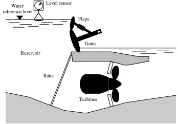
Figure 1: Configuration of the river power plant
paper we consider the hydro power plant described in [7, 8] that includes three types of water outflow units: Four gates, four flaps and two turbines. The weirs (i.e. gates and flaps) form a barrage across the river (see Figure 1) and the total outflow of the dammed river is determined both by the water level in the reservoir and by the opening of the units. The manipulated vari-ables are the openings of each outflow element and the measured variables are the total outflow and the power generated.
There are three main reasons why the outflow units are suitably modeled as hybrid systems [13, 5]. First, the actuator action is given by a discrete input to the step-per motors of the components, namely the commands to open, close, or leave unchanged the opening of the outflow element. Second, the internal description of every element is a finite state machine that associates different opening dynamics to different logical states. Finally, the plant operation is strongly influenced by qualitative decision rules about the use of one type of outflow unit rather than another one. For instance if the desired outflow increases, the controller should first try to increase the flow through the turbines, rather than the openings of the weirs, in order to maximize the produced power. A less trivial constraint is that the procedure of opening and closing an outflow ele-ment cannot be arbitrarily short. If an outflow eleele-ment has started to move, it should be kept on moving for a given minimal time.
relation logic mixed integer inequalities
P1 AND S1∧S2 δ1= 1
(∧) δ2= 1
P2 S3↔ −δ1+δ3≤0
S1∧S2 −δ2+δ3≤0
δ1+δ2−δ3≤1
P3 OR (∨) S1∨S2 δ1+δ2≥1
P4 NOT(∼) ∼S1 δ1= 0
P5 IMPLY (→) S1→S2 δ1−δ2≤0 P6 [aTx≤0]→[δ= 1] aTx≥ǫ+ (m−ǫ)δ
P7 [δ= 1]→[aTx≤0] aTx≤M−M δ
P8 IFF (↔) S1↔S2 δ1−δ2= 0
P9 [aTx≤0]↔[δ= 1] aTx≤M−M δ aTx≥ǫ+ (m−ǫ)δ
P10 Product z=δ·aTx z≤M δ
−z≤ −m δ z≤aTx−m(1−δ)
−z≤ −aTx+M(1−δ)
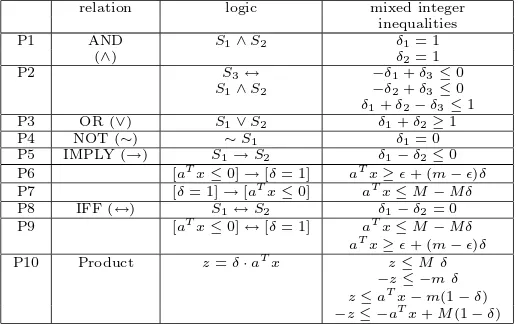
Table 1: Basic conversion of logic relations into mixed-integer inequalities.
to solve fault detection and state estimation problems within a receding horizon estimation scheme [9].
In Section 2 a concise introduction to MLD systems is given, showing the main steps for deriving MLD models of plants. The modeling procedure is then detailed in Section 3 with reference to the model of the flaps, that are the simplest outflow units of the plant considered. A simulation of the flap unit is reported in Section 4 and the main issues regarding the control of the overall plant are discussed in Section 5.
2 Hybrid Systems in the MLD Form
The derivation of the MLD form of an hybrid systems involves basically three steps [4]. The first one is to as-sociate with a statement S, that can be either true or false, a binary variable δ∈ {0,1} that is 1 if and only if the statement holds true. Then, the combination of elementary statements S1, . . . , Sq into a compound
statement via the boolean operators and (∧), or (∨), not (∼) can be represented as linear inequalities over the corresponding binary variablesδi,i= 1, . . . , q. The
inequalities stemming from the basic compound state-ments are reported in Table 1. As an example consider P3, which says that the statementS1∨S2 holds true if
and only ifδ1 andδ2sum up at least to one.
A special statement is given by the conditionaTx≤0,
wherex∈X⊆Rnis acontinuous variable1andXis a
compact set. If one definesmandM as lower and up-per bounds on aTxrespectively, the inequalities in P9
assign the valueδ= 1 if and only if the value ofx sat-isfies the threshold condition. Note that in P6 and P9,
ǫ >0 is a small tolerance (usually close to the machine
1
We call a variable continuous when it takes values in an
infinite set
precision) introduced to replace strict inequalities by non-strict ones.
The second step is to represent the product between linear functions and logic variables by introducing an auxiliary variablez=δaTx. Equivalently,zis uniquely
specified through the mixed-integer linear inequalities inP10.
The third step is to include binary and auxiliary vari-ables in an LTI discrete-time dynamic system in order to describe in a unified model the evolution of the con-tinuous and logic components of the system.
The general MLD form of a hybrid system is [4]
x(t+ 1) =Ax(t) +B1u(t) +B2δ(t) +B3z(t) (1a)
y(t) =Cx(t) +D1u(t) +D2δ(t) +D3z(t) (1b)
E2δ(t) +E3z(t)≤E1u(t) +E4x(t) +E5 (1c)
wherex= [xTc xTℓ]T ∈Rnc×{0,1}nℓ are the continuous
and binary states,u= [uTc uTℓ]T ∈Rmc× {0,1}mℓ are
the inputs,y = [yT
c yℓT]T ∈Rpc× {0,1}pℓ the outputs,
and δ ∈ {0,1}rℓ, z ∈ Rrc represent auxiliary binary
and continuous variables respectively. All constraints on the state, the input,zand theδvariables are sum-marized in the inequality (1c). Note that, although the description (1) seems to be linear, nonlinearity is hidden in the integrality constraints over the binary variables.
MLD systems are a versatile framework to model var-ious classes of systems. For a detailed description of such capabilities we defer to [4, 1]. In this paper we will focus on the capability of MLD systems for describ-ing automata, systems driven by a discrete-input and Piece-Wise Affine (PWA) relations. From the guide-lines of this Section, it should be apparent that the procedure for representing a hybrid system in the MLD form (1) can be automatized. A compiler (HYSDEL - HYbrid System DEscription Language) that gener-ates the matrices of the MLD system starting from a high-level description of the system is currently in Beta-testing at ETH Z¨urich [2].
3 The Models of the Units
The openings of the turbines and the weirs control the total outflow of the hydroelectric power plant. An outer loop with a simple PI regulator usually controls the level of the water in the reservoir [14]. This level, denoted by uc in Figure 2, is a continuous input to
the system formed of flaps and gates. The openingα
the connected electric network: In this case the tur-bines must be closed as fast as possible and the weirs must be opened quickly to maintain the global outflow constant. For sake of simplicity, in Figure 3 we omitted the obvious transitions from one state to itself.
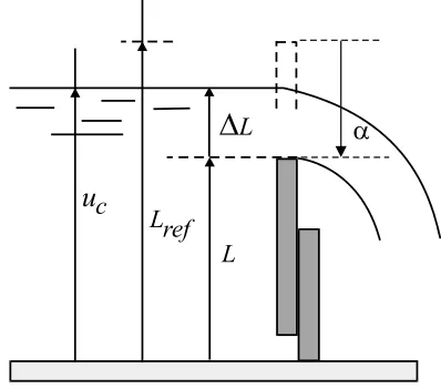
Figure 2:Parameters characterizing the outflow of a flap.
Figure 3: Automaton of the stepper motor.
The stepper motor is driven by a discrete inputuℓ(t)∈
{open, close, stop, emergency} that controls the
transitions between the five logical states Opening, Closing, Stop, Emergency and , Stand-by. In order to derive an MLD representation of the stepper motor, we have to code the logical states and the in-puts into vectors of binary variables. In principle, it is possible to associate with each different state/input a new binary variable , but this procedure would increase the computational burden for the simulation (and the control) of the model [4]. Therefore, we use the min-imal number of logical variables, i.e. two logic input variablesuℓ,1, uℓ,2 and three logic state variablesxℓ,1,
xℓ,2,xℓ,3that code the discrete inputs and states of the
automaton as in Tables 2 and 3.
Note that, as depicted Figure 3, the admissible
tran-stop open close emergency
uℓ,1 0 1 0 1
uℓ,2 0 0 1 1
Table 2:Coding of the logical inputs of the stepper motor
Stop Opening Closing Emergency Stand-by
xℓ,1 0 1 0 1 1
xℓ,2 0 0 1 1 1
xℓ,3 - - - 0 1
Table 3:Coding of the logical states of the stepper motor. The symb ol ’ - ’ denotes indifferently 0 or 1.
sitions depend also on the value of α that is con-strained between the minimum and maximum opening (αmin = 0 [m] and αmax = 2 [m]). For instance, the
transition fromstopto openingis not allowed if the weir is completely opened (i.e. α=αmax) even if the
commandopenoccurs. To take into account these con-ditions, we introduce two logical variablesδmax(t) and
δmin(t) defined by
[δmax(t) = 1] ↔ α(t)≥αmax (2)
[δmin(t) = 1] ↔ α(t)≤αmin (3)
To model the evolution of the logical state xℓ(t), it is
convenient to introduce three logical variables δℓ,1(t),
δℓ,2(t),δℓ,3(t) defined asδℓ,i(t) =xℓ,i(t+ 1),i∈1,2,3.
With the notations introduced so far, every state tran-sition of the automaton depicted in Figure 3 can be described as a logical implication. For instance, the transition from the state Open at time t to Stop at timet+ 1 is modeled as
In order to find the linear inequalities representing (4) one has two possibilities. The first one is to re-write (4) inConjunctive Normal Form (CNF) and then use the rules of Table 1 to compute the system of inequalities. Alternatively, one can use the algorithm described in [15] that allows computing the inequalities in an auto-mated way directly from the truth-table of proposition (4).
The dynamics of the openingαdepends on the logical state of the stepper motor
˙
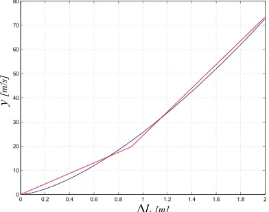
Figure 4: Approximation of the outflow profile.
provided that the new logical variablesδo,δc,δeare set
equal to one when the values of the logical states, the logical inputs and the saturation indicators δmax and
δmin allow opening or closing the weir. For instance,
the value ofδeis assigned by the proposition
The last task is to compute the outflow that is the output of the system. For this purpose we describe the outflow of a flap. The case of a gate is conceptually almost identical. The outflow law is given by [12]:
y(t) =
river and the opening of the flap (as depicted in Fig-ure 2), Lref = 7.5 [m] and CD = 0.6 is the discharge
coefficient. From (7) it is apparent that the outflow is a nonlinear function of ∆L. In order to embed (7) in the MLD form (1) we have to approximate it either in a lin-ear or piecewise affine way. By using a linlin-ear function it was impossible to reduce the maximum error below 10.63% in the range of interest for ∆L. To reduce the error, we approximate (7) with the piecewise affine function depicted in Figure 4, thus obtaining a maxi-mum error of 3.31%. Then, the approximated outflow is described by the equations
y(t) =
PWA function (8) can be incorporated into the MLD
equations in the following way. First, we introduce the logical variables
[δlin1= 1] ↔ [∆L≥0] (9)
[δlin2= 1] ↔ [∆L≤p] (10)
[δlin3= 1] ↔ [∆L≥p] (11)
and write the outflow as
y(t) = 0·(1−δlin1)δlin2(1−δlin3) +m1∆y(t)·δlin1δlin2(1−δlin3) + +(m2∆y(t) +p(m1−m2))·δlin1(1−δlin2)δlin3 (12)
Then, we introduce the binary variable δlin(t) =
δlin1(t)δlin2(t) (the corresponding inequalities can be
derived from P2 in Table 1) and the auxiliary variables
zlin1(t) =δlin(t)uc(t), zlin2(t) =δlin(t)α(t),
zlin3(t) =δlin3(t)uc(t), zlin4(t) =δlin3(t)α(t). (13)
Finally, we obtain the expression
y(t) =m1zlin1(t) +m1zlin2(t) +m2zlin3(t) +m2zlin4(t)
−Lrefm1δlin(t) + (p(m1−m2)−m2Lref)δlin3(t) (14)
To summarize the results obtained so far, the over-all MLD model, for a single flap is described by the variables
The 125 inequalities stemming from the representation of the δ and z variables are collected in the matrices
Ei,i= 1, . . . ,5 of (1c) and are not reported here due
to the lack of space.
By using the methodology outlined in Section 3, one can also derive the MLD description of the gates and the turbines. Details are available in [6]. We only sum-marize the main modeling issues. The model of the gates differs from the one of the flaps only in the ap-proximation of the outflow law that is
Figure 5: Automaton of the turbine.
and depends in a nonlinear way both onα(t) anduc(t).
Concerning the turbines, depicted in Figure 5, one has to take into account also the start and stop procedures that involve the presence ofclocks. In the MLD frame-work, clocks can be modeled by introducing additional states and they can be initialized by properly modeling the resetting logic. For a turbine, one must also com-pute the produced power (that depends on the outflow, among other variables) as additional output. Usually, this nonlinear relation between the opening of the tur-bine, the head and the outflow is provided by the man-ufacturer of the turbine in the form of a lookup table. Then, one has to approximate the lookup table with a PWA function keeping in mind that the finer the approximation, the more complex (in terms of binary variables) the overall model.
4 Simulation of the flap model
The MLD system derived in the previous section is
completely well-posed [4] meaning that at each time instant, the maps (x(t), u(t))→δ(t) and (x(t), u(t))→
z(t) are single-valued. This property, that is usu-ally verified when representing real plants in the MLD form, plays an important role for the simulation. In-deed, for completely well-posed systems, given the pair (x(t), u(t)) it is possible to determine the values of
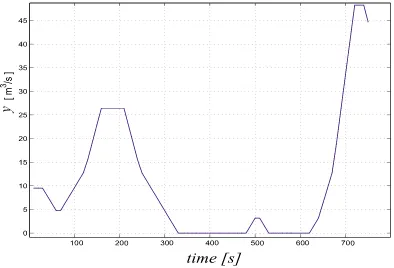
δ(t) and z(t) by solving a Mixed-Integer Feasibility Test w.r.t. the constraints (1c). This test can be done very efficiently by using Branch and Bound al-gorithms [16, 10, 3]. For instance, the simulation pre-sented in Figure 6 was computed in 11.23s on a Sun Sparc Ultra60 Workstation running Matlab5.3. The simulation in Figure 6 was obtained by keeping the water level in the reservoir constant (uc(t) = 7 [m]),
and setting the initial conditions asα(0) = 1 [m] and
xℓ(0) =Stop. The corresponding outflow profile is
de-picted in Figure 7. In Figure 6, for representing the sequence of logical inputs we associate the value 1 with
open, the value 0 with stop, the value -1 withclose
and the value -2 withemergency. We excited the sys-tem in such a way to show its behavior in many op-erating conditions. For instance, when theemergency
signal occurs , the flap correctly opens up to αmax at
the fast speedTcτe ignoring the input applied at the next time samples.
Figure 6:Simulation of the flap opening. Squares: open-ingα(t+ 1), Crosses: logical inputuℓ(t).
Figure 7: Outflow profile.
5 Outflow control
As described in the introduction, the controller chooses which outflow element has to be manipulated in or-der to control the total outflow. The decision should maximize the total power generation while taking into account several qualitative priorities. For instance, in nominal operating conditions these are:
• open turbines rather than gates
• open turbines rather than flaps
The complete list of such priorities is given in [7]. For systems in MLD form these priorities can be expressed as mixed integer linear inequalities and they can be modeled as additional constraints in the MPC scheme [4, 11].
The control algorithm is applied to the overall plant, which is obtained by aggregating the single outflow units. For nominal operation however, the complexity of the components modeled in Section 3 is unnecessar-ily high. For instance, there is no need to model the emergency signals since emergencies are very unlikely to be handled by the MPC scheme in an automated way.
The control problem requires the solution of a mixed integer quadratic program at each time step. The use of simplified models allows also to improve the speed of the numerical computations involved for the controller synthesis. The complexity of such problems depends mainly on the number of binary variables in the model. To improve the efficiency of the control algorithm, we have built up models of lower complexity in terms of the total number of binary variables.
Both the simplified models of the overall plant and sim-ulation results for the control scheme will be included in the final version of the paper.
6 Conclusions
In this work we model the outflow units of a hydro-electric power plant in the framework of Mixed Logic Dynamical (MLD) systems. This opens the way to the design of model predictive control algorithms that, be-side tracking the desired outflow, can take into account prioritized specifications.
Acknowledgments
The authors thank Dr. J. Chapuis for the fruitful dis-cussions. This research is supported by the Swiss Na-tional Science Foundation.
References
[1] A. Bemporad, G. Ferrari-Trecate, and M. Morari. Observability and Controllability of Piecewise Affine and Hybrid Systems.IEEE Transactions on Automatic Control, 2000.
[2] A. Bemporad, P. Hertach, D. Mignone, M. Morari, and F.D. Torrisi. HYSDEL- Hybrid Systems Description Language. Technical report, ETH-Z¨urich, 2000.
[3] A. Bemporad, D. Mignone, and M. Morari. An Efficient Branch and Bound Algorithm for State Es-timation and Control of Hybrid Systems. European Control Conference, 1999.
[4] A. Bemporad and M. Morari. Control of Systems Integrating Logic, Dynamics, and Constraints. Auto-matica, 35(3):407–427, March 1999.
[5] M.S. Branicky. Studies in Hybrid Systems: Mod-eling, Analysis, and Control. PhD thesis, Massachus-sets Institute of Technology, 1995.
[6] D. Castagnoli. Modellizzazione di una centrale idroelettrica ad acqua fluente mediante sistemi ibridi. Universit´a degli Studi di Pavia, 2000. Forthcoming Master’s thesis.
[7] J. Chapuis. Modellierung und neues Konzept f¨ur die Regelung von Laufwasserkraftwerken. Diss. ETH Nr. 12765, ETH Z¨urich, 1998.
[8] J. Chapuis and F. Kraus. Application of fuzzy logic for selection of turbines and weirs in hydro power plants. InProc. 14th IFAC World Congress, 1999. [9] G. Ferrari-Trecate, D. Mignone, and M. Morari. Moving Horizon Estimation for Piecewise Affine Sys-tems.Proceedings of the American Control Conference, 2000.
[10] C.A. Floudas. Nonlinear and Mixed-Integer Op-timization. Oxford University Press, 1995.
[11] E.C. Kerrigan, A. Bemporad, D. Mignone, M. Morari, and J. M. Maciejowski. Multi-objective Pri-oritisation and Reconfiguration of Hybrid Systems us-ing Model Predictive Control.Proceedings of the Amer-ican Control Conference, 2000.
[12] G. Krivchenko. Hydraulic Machines: Turbines and Pumps - Second Edition. Lewis Publishers, 1994. [13] G. Labinaz, M.M. Bayoumi, and K. Rudie. A Survey of Modeling and Control of Hybrid Systems.
Annual Reviews of Control, 21:79–92, 1997.
[14] M. Lahlou.Mod´elisation des canaux hydrauliques et application au r`eglage de niveau. Institut d’ ´electronique industrielle., EPF Lausanne, Switzerland, 1994.
[15] D. Mignone, A. Bemporad, and M. Morari. A Framework for Control, Fault Detection, State Estima-tion and VerificaEstima-tion of Hybrid Systems. Proceedings of the American Control Conference, 1999.