ANALYSIS
The assumption of equal marginal utility of income: how
much does it matter?
Hege Medin
a,1, Karine Nyborg
a,*, Ian Bateman
b aDi6ision for En6ironmental and Resource Economics,Research Department,Statistics Norway,P.O.Box8131Dep.,
N-0033Oslo,Norway
bCentre for Social and Economic Research on the Global En6ironment(CSERGE),School of En6ironmental Sciences, Uni6ersity of East Anglia,Norwich NR4 7TJ,UK
Received 7 February 2000; received in revised form 9 August 2000; accepted 9 August 2000
Abstract
In most applied cost – benefit analyses, individual willingness to pay (WTP) is aggregated without using explicit welfare weights. This can be justified by postulating a utilitarian social welfare function along with the assumption of equal marginal utility of income for all individuals. However, since marginal utility is a cardinal concept, there is no generally accepted way to verify the plausibility of this latter assumption, nor its empirical importance. In this paper, we use data from seven contingent valuation studies to illustrate that if one instead assumes equal marginal utility of the public good for all individuals, aggregate monetary benefit estimates change dramatically. © 2001 Elsevier Science B.V. All rights reserved.
Keywords:Utility comparisons; Cost – benefit analysis; Choice of numeraire; Environmental goods JEL classification:D61; D62; D63; H41; Q2
www.elsevier.com/locate/ecolecon
1. Introduction
Undergraduate students of economics usually spend considerable time and energy grappling
with the concept of ordinal utility. This is not surprising given that ordinal utility is not com-parable between persons and does not tell us anything about intensities, being simply a tool for describing an individual’s binary choices. As such, it is a concept very much deprived of normative content (Sen, 1977), although it is extremely use-ful for purely descriptive analyses.
When faced with the task of conducting an applied cost – benefit analysis after graduation,
* Corresponding author. Tel.: +47-22-864868; fax: + 47-22-864963.
E-mail addresses: [email protected] (K. Nyborg), [email protected] (I. Bateman).
1Present affiliation: Norwegian Institute of International Affairs, P.O. Box 8159 Dep, N-0033 Oslo, Norway
however, many economists need to go through the reverse process, since applied cost – benefit analy-sis requires acardinal, interpersonally comparable utility concept (Arrow, 1951). After spending so much time getting accustomed to ordinal utility, the economist now has to grasp the implicit con-sequences of assuming, instead, that utility does indeed tell us something about intensities, and that onecan compare benefits between persons.
There is currently no generally accepted way to measure cardinal and interpersonally comparable utility. In applied cost – benefit analysis, the most common way to proceed is to use the unweighted sum of individuals’ net willingness to pay as a measure of social benefits. This is consistent with using a utilitarian social welfare function along with an assumption of equal marginal utility of income for all individuals. However, since the latter assumption does not rest on any empirical evidence, it introduces a certain kind of arbitrari-ness into the analysis. Unlike the choice of social welfare function, which can be discussed on ethi-cal grounds, assumptions about the cardinality and comparability aspects of utility functions may be regarded as positive rather than normative; but the problem is that, in the absence of measure-ment methods, these assumptions cannot be em-pirically verified. One simply does not know whether the assumption of equal marginal utility of income is reasonable.
However, although we cannot directly test the plausibility of this assumption, we may still per-form sensitivity analyses regarding the robustness of results to alternative ways of comparing cardi-nal utility between persons. This paper is an at-tempt to do precisely that. Based on data from seven contingent valuation (CV) studies of envi-ronmental changes, we calculate aggregate mone-tary benefits using an alternative operationalisation of cardinal and interpersonally comparable utility, namely, that individuals have an equal marginal utility of the environmental good in question.
This latter assumption corresponds to using units of the environmental good as the numeraire when aggregating individual benefits, instead of the usual approach of using money for this pur-pose. Until recently, it was a common belief that
the choice of numeraire does not matter in cost – benefit analysis. However, Brekke (1997) demon-strated that the unit of measurement did indeed matter (see also Dre´ze, 1998; Johansson, 1998). Brekke pointed out that, when it comes to public goods, different individuals generally have differ-ent marginal rates of substitution, since the amount of the public good is necessarily equal for all; implying that individuals have different mar-ginal conversion rates between those goods that may alternatively be chosen as the numeraire. Consequently, when individual benefit estimates are aggregated, the interests of different individu-als are given a different emphasis depending on which measurement unit is used.
Brekke’s result may be dismissed as irrelevant by some, arguing that it is not practicable to use environmental units. For example, one cannot always in practice pay compensations in environ-mental units2, and survey questions using
environ-mental units may be very difficult for respondents to understand. However, we believe that the im-portance of Brekke’s result lies elsewhere. As al-ready mentioned, using environmental units as the numeraire corresponds to an alternative opera-tionalisation of cardinal, interpersonally compara-ble utility. As such, it provides a means to check the empirical importance of the seemingly innocu-ous, but admittedly arbitrary, assumption of equal marginal utility of income used in most applied cost – benefit analyses. Brekke presents one empirical example in his paper. Using data from a survey by Strand (1985), he found that the maximum per person cost that would make the project’s net benefits positive were 22times higher
if money were used as a numeraire than if one used environmental units. In other words, ex-changing the assumption of equal marginal utility of income for an assumption of equal marginal utility of the public good changed the result dra-matically in this particular case. It is hard to see that the former assumption is more plausible than the latter from a theoretical point of view: Argu-ing in favour of one or the other requires reason-ing about cardinality and interpersonal
comparisons of utility, which is rarely found in economic theory. However, apart from Brekke’s own example, we know of no attempts in the literature to analyse empirically the sensitivity of aggregate benefit estimates with respect to the choice of assumptions concerning marginal utilities.
The widespread use of aggregate unweighted WTP as an estimate of social benefits has been criticised by many scholars (for example, Kelman, 1981; Bromley, 1990; Hammond, 1990; Vatn and Bromley, 1994). If alternative and seemingly equally a priori plausible ways to operationalise interpersonally comparable cardinal utility yielded dramatically different results than the standard procedure, this should be of concern for all practi-tioners and users of cost – benefit analysis. In such a case, the traditional assumption cannot be de-fended by convenience alone, and one needs to take the issue of interpersonal comparisons of utility more seriously. We believe, therefore, that it is important to investigate whether Brekkes’ finding of dramatically different aggregate benefit estimates holds more generally.
We should stress at the outset, however, that our aim is neither to argue that using environmen-tal units is necessarily more relevant than using money as a numeraire, nor to identify the ‘best’ way to aggregate individual welfare. We recognise that money, being a much more generally ex-changeable numeraire than environmental units, is the most convenient measurement unit in many contexts. Under certain conditions, it may also be argued that assuming equal marginal utility of money is more reasonable than assuming equal marginal utility of the public good. For example, if there are respondents with negative WTPs, the latter assumption would imply that some people have a negative marginal utility of money, which seems implausible. As discussed below, however, there are also conditions under which equal mar-ginal utility of the public good is the most reason-able assumption of the two. Rejection of one of these assumptions does not imply that the other is correct. Maybe both are wrong. Given that we do not know how to measure interpersonally com-parable cardinal utility, we are simply examining
the empirical implications of replacing current practice with an alternative approach that is, in theory, equally valid. Our result is, in brief, that the two methods yield very different results.
2. Some central concepts
Below, we present a simple model explaining the main concepts which will be used in our calculations. The reader is referred to Brekke (1993, 1997), Medin (1999) for further details.
2.1. Aggregating net willingness to pay
Assume that there are n heterogeneous con-sumers with utility functions
Ui=ui(Yi,E) (1)
for all i=(1, …, n), where Yi is individual i’s
income, and E is a pure public good, which we will think of as being provided by the environ-ment. E will be measured in physical units, for example, the estimated number of fish in a lake, or km2
of wilderness. Utility is assumed to be increasing in income and the public good.
Consider a project where the environmental good is increased by dE\0, at a total cost SCi,
where Ci is the amount of money personi has to
pay if the project is implemented. To avoid com-plicating matters unnecessarily, we will assume that Ci= −dYi=C for every i=(1, …, n), i.e.
every individual faces the same cost. A money measure dUiY of the project’s net effect on i’s
utility can be derived by differentiating Eq. (1) and dividing by the individual’s marginal utility of income, uiY:
dUi
Y
=uiE
uiY
dE−C=WTPidE−C (2)
whereuiEis the individual’s marginal utility of the
public good. WTPi is the indi6idual’s marginal
gross willingness to pay for the environmental
improvement, and dUi
Y is her net willingness to
minus the costs she has to pay,C).3 We will take
as a starting point that C and dE are known. Individuals’ marginal rates of substitution uiE/uiy
can in principle be observed by asking their willing-ness to pay for a one unit change in the environ-mental good; below, we will abstract from all practical problems of actually eliciting true willing-ness to pay, and simply assume that it can be observed. Assume further that social welfareWcan be written as a differentiable function of individual utilities:
W=V(U1(Y1,E), …,Un(Yn,E)) (3)
Assume that the project is marginal for all individuals, in the sense that any changes in individ-uals’ marginal rates of substitution due to the project’s implementation are small enough to be disregarded. Then, the project’s effect on social welfare is
dW= %
n
i=1
{Vi(uiYdYi+uiEdE)}= % n
i=1
(ViuiYdUiY)
(4)
whereVidenotes the partial derivative of the social
welfare function with respect to personi’s utility. In applied cost – benefit analysis, explicit welfare weightsViuiY are rarely used (Little and Mirrlees,
1994). The most common procedure is simply to estimate social benefits as the unweighted sum of individuals’ net willingness to pay, which is consis-tent with Eq. (4) only ifViuiY=VjujY for alli,j.
4
If the social welfare function is such thatVishould
always be inversely proportional to i’s marginal
utility of income, equality of welfare weightsViuiY
will, of course, always hold.5 Generally, however,
these welfare weights depend on the marginal utility of income. For example, if we use a utilitarian social welfare function, the net willingness to pay of individuals with a high marginal utility of income should get a larger weight in the cost – benefit analysis than others. However, as there is no generally accepted method to measure the marginal utility of income in an interpersonally comparable way (although some measurement at-tempts have certainly been made; see Frisch, 1932; van Praag, 1991), it is virtually impossible to verify the assumptions one makes on this parameter.
Some economists have argued that efficiency and distribution are two separate issues which could and should dealt with separately (e.g. Hicks, 1939), and defend unweighted aggregation of net willing-ness to pay on that ground. However, such reason-ing usually relies on the assumption that costless lump-sum redistribution of income is available, which is rarely the case in large economies with private information (Hammond, 1979).6
Un-weighted aggregation of net willingness to pay may further be justified by assuming that the status quo income distribution is socially optimal. Note, how-ever, that not only would a decision-maker need an extreme degree of power to actually implement the income distribution of her choice, she would also encounter exactly the same problem of non-observ-ability as the cost – benefit analyst. In order to identify the social optimum, the decision-maker too must know every individual’s interpersonally com-parable marginal utility of incomeuiY. It is not clear
how such information, which is unobservable for the analyst, could be available to decision-makers.7 3Note the difference between gross and net willingness to
pay. In the latter, costs are deducted. Here, dUiYisi’s
compen-sating variation for the entire project (costs taken into ac-count). For a project in which dEB0, dUiYwould correspond
to the equivalent rather than compensating variation. How-ever, the difference between compensating variation and equiv-alent variation does not matter for marginal projects under standard neoclassical assumptions. For a critical discussion of the latter with respect to such welfare measures, see Bateman et al. (1997a).
4Strictly speaking, it is consistent with Eq. (4) only if ViuiY=1 for alli. However, if we have insteadViuiY=Kfor
all i, whereK\0, the choice of the constant K would not
matter for the ranking of projects.
5This implies that if the marginal utility of income decreases in income, an individual’s interests receivesmoreweight in the social welfare function the richer he is.
6Dre`ze and Stern (1987) discuss several arguments for the view that distributional concerns can be disregarded in a cost – benefit analysis, and reject all of them. Their conclusion is that explicit welfare weights should be used in cost – benefit analysis, for example, by estimating the welfare weights im-plied by earlier policy deicisions.
2.2. Aggregating public good requirements
Above, individual utility changes were measured in monetary units. Quite equivalently, one may measure utility changes using some other nu-meraire than money. In our simple two-good model, thus, individual utility changes may alterna-tively be measured using units of the environmental good. Differentiation of the utility function (Eq. (1)) and dividing byuiEyields a measure of
individ-ual net benefits in environmental units, dUE:
dUi
environmental good individualidemands in order to be willing to payC. We will call this measurei’s
public good requirement. By differentiating Eq. (3)
it can easily be seen that net social benefits may be expressed as a function of individuals’ net benefits in environmental units (Brekke, 1997):
dW= %
n
i=1
(ViuiEdUiE) (6)
Corresponding to the case of monetary units, simple unweighted aggregation of individuals’ net benefits in environmental units requires that
ViuiE=VjujEfor alli,j. Again, these weights depend
on unobservable aspects of individual utility, and cannot generally be determined through knowledge of the social welfare function alone.
2.3. Marginal utility: two alternati6e assumptions
In the following, we will replace Eq. (3) by a utilitarian social welfare function:
W= %
n
i=1
Ui (7)
This simplifies the calculations and makes the analysis more transparent, allowing us to focus on utility measurement and comparability rather than the social objective function itself.8Note, however,
that although our empirical results would look different with another choice of social welfare function, the problems posed by unobservability of cardinal and interpersonally comparable utility would not disappear.
We have chosen to study two particularly simple assumptions concerning cardinal utility.
Alternative I
The marginal utility of income is equal for all. This would, for example, hold if a utilitarian and omniscient decision-maker had already redis-tributed income to implement a socially optimal income distribution. It would also hold if the level of income were equal for every consumer, and utility functions were of the following additively separable form:
Ui=f(Yi)+gi(E) (8)
Alternative II
The marginal utility of the public good is equal for all. This would, for example, always hold, regardless of individual income levels, if utility functions were of the following additively separable form:
Ui=fi(Yi)+g(E) (9)
Under Alternative I, a money measure of social benefits dWYcan be derived by unweighted
aggre-gation of net willingness to pay (alternatively, unweighted aggregation of gross willingness to pay minus aggregate costs), such that the project is welfare-improving if dWY\0.
dWY= This corresponds to the net benefit estimate from a standard unweighted cost – benefit analysis.
Under Alternative II, unweighted aggregation of individual net benefits in environmental units yields a social benefit estimate dWE
, measured in envi-ronmental units. If this indicator is positive, the increase in the environmental good is large enough to justify the costs nC.
dWE
While the indi6idualnet benefit estimators dU i Y
and dUiE will always have the same sign as the 8The utilitarian moral philosophy has been popular among
individual’s utility change, regardless of the chosen numeraire, the aggregate benefit estimators dWY
and dWEmay have different signs (Brekke, 1997).
This is caused by the different assumptions about interpersonal comparability of cardinal utility un-derlying these indicators. Changing the way one operationalises interpersonal comparisons of utility is equivalent to a change of normative weightsVi.
2.4. Maximum acceptable costs
Apart from the possibility of different signs, it is difficult to use dWY
and dWE
directly to judge the empirical importance of a particular choice of aggregation method. They are measured in differ-ent units, and since each person may have a different ‘exchange rate’ between units (i.e. differ-ent marginal rates of substitution), it is not obvious which conversion rate one should use in an attempt to make them directly comparable. However, an interesting comparison can be made by looking at
the per person costs which would lea6e the project
with exactly zero net benefitsusing the two methods.
If we denote byC* the per person cost that implies dWY=0, i.e. the maximum acceptable per person
cost when equal marginal utility of income is assumed, we have from Eq. (10) that
C*=1
Similarly, we can denote byC** the maximum allowable per person cost when equal marginal utility of the environmental good is assumed.C** can be defined by
C**= n
which is the per person cost implying exactly dWE
=0. C* and C** can both be regarded as monetary measures of aggregate benefits from increasing the public good supply.9
An interesting indicator for the empirical impor-tance of the choice of numeraire is C*/C**. This will be the central indicator in our empirical results. We will denote this the maximum acceptable cost (MAC) ratio. Mathematically, the MAC ratio is given by It can easily be seen from Eq. (14) that if all individuals have the same marginal rate of substi-tution between income and the environmental good, the MAC ratio=1. Hence, if we are con-cerned only with ordinary market goods in a perfectly competitive market (assuming no corner solutions), the maximum acceptable per person costs will be the same using both measurement methods. However, whenever marginal rates of substitution differ between individuals, the nu-meraire problem will arise. This will be the case in a number of circumstances, e.g. when some goods are rationed (see Dre´ze, 1998); but for simplicity, we will concentrate on the case where the good is a public (environmental) good.
For later reference, we note that Eq. (14) could alternatively be expressed as (see also Eqs. (2) and (5)):
is the average of all respondents’ marginal willing-ness to pay, and
WTP−1
is the average of all respondents’in6ersewillingness
to pay. Thus, even if we do not have direct information on people’s public good requirements, MAC ratios can be calculated using individual willingness to pay data only, assuming that the project is marginal.10The MAC ratios reported in
the next section were calculated using Eq. (15).
9Note the similarity to the uniform variation measures proposed by Hammond (1994). The uniform compensating variation is defined as the total amount that society is willing to pay, in the form of a uniform poll tax on all individuals, in order to be allowed to move from the status quo to an alternative social state.
Generally, a given numeraire will favour the interest of a person if the numeraire is of rela-tivelylow value to that person (Brekke, 1997). If, for example, a person only gets a relatively small utility increment from receiving an extra dollar, this person’s net benefits of a project expressed in money terms must become a large number. How-ever, if the same person gets a relatively high utility increment of an extra unit of the public good, her net benefits expressed in environmental units must be a small number. Consequently, using money as the numeraire will favour those with a relatively high valuation of the environ-ment compared with using environenviron-mental units as the numeraire.
The MAC ratio presupposes that costs are shared equally between individuals. Under this assumption, unless the project is a Pareto im-provement, those who have the lowest valuation of the environmental good will always be the project’s opponents because the cost they have to pay always exceeds their willingness to pay. Thus, the benefit measure C* will systematically give less weight to the interests of the project’s oppo-nents thanC**, implying that the MAC ratio ]1
will always hold.11 In other words, given the
assumptions employed here, assuming that every-body has the same marginal utility of income will
always fa6our the project, compared with the
alter-native assumption of equal marginal utility of the public good.
The indicators presented above presuppose that the project can be regarded as marginal. If the
project is non-marginal in the sense that individu-als’ marginal rates of substitution change signifi-cantly due to the project’s implementation, the above indicators provide only approximations. However, regarding the MAC ratio, errors caused by changes being non-marginal will generally go in both directions because the public good re-quirement is overestimated for those who have positive net benefit from the project and underes-timated for those who have negative net benefit from the project. We thus cannot know a priori whether the MAC ratio is over- or under esti-mated in the case of a non-marginal public good change. In the special case of quasi-linear utility, however, the MAC ratio will be correct even if the public good change is non-marginal.12
3. Empirical results
The disturbing part of the theoretical results discussed above is that one way of operationalis-ing cardinal and interpersonally comparable
util-ity systematically favours certain interest groups,
compared with another, equally simple method. However, if this bias was of a small empirical magnitude, it might still not be of much practical importance. To examine the empirical significance for applied cost – benefit analysis of the choice of assumption regarding cardinal utilities, we have calculated the MAC ratio from seven contingent valuation studies using individual willingness to pay data. Unfortunately, our results indicate that the choice of numeraire (corresponding to a cer-tain choice of assumption on cardinal utilities) may be extremely important.
3.1. Data
The studies we have used are those of Loomis (1987), Navrud (1993), Bateman and Langford (1997), Bateman et al. (1995, 1997b), Magnussen et al. (1997), Strand and Wahl (1997). All the studies examine willingness to pay to avoid reduc-tions in certain specified recreational services,
ex-11It is possible to calculate similar indicators with other assumptions concerning the distribution of costs. A more generally applicable indicator may be denoted the TMAC ratio, the ratio of maximum allowable total costs, where TMAC=MAC ifCi=Cfor everyi. One will generally have a
TMAC ratio \1 if costs are shared ‘under-proportionally’ with individual marginal willingness to pay for the environ-mental good, i.e.Ci=K(uiE/uiY)
a
, whereKandaare positive constants, and aB1. Equal distribution of the costs is a special case of under-proportionally cost distribution. If costs are ‘over-proportionally’ distributed (a\1), we get a TMAC ratioB1. However, overproportional cost sharing seems to be
a fairly peculiar sharing rule, leading to severe incentive com-patibility problems. Proportional cost distribution will give a TMAC ratio=1 (see Brekke, 1993; Medin, 1999 for detail on this issue).
cept the Magnussen et al. (1997), Bateman and Langford (1997) surveys, which measure willing-ness to pay for an increase in recreational ser-vices.13 Several of the studies varied the survey
design between subsamples; for those studies, re-sults are reported for each subsample. The table below reports results for a total of 18 subsamples. A brief summary of each study is provided in Medin et al. (1998), (Appendix 2). All calculations are based on open-ended WTP data.14
3.2. Outliers and zero bids
A well-known problem in contingent valuation research is that average WTP estimates, and thus
C*, can be sensitive to extremely high reported individual values. A common approach to such ‘outliers’ is simply to omit them from the data assuming that they are caused by errors, misun-derstandings, strategic responses, or protest reac-tions on respondents’ part. On the other hand, if these ‘extreme’ observations do reflect respon-dents’ valuations, one may obviously understate average (and aggregate) willingness to pay by omitting them.
When environmental units are used as nu-meraire in the aggregation of individual welfare effects, one encounters a similar problem regard-ing extremely low observations of individual will-ingness to pay (low uiE/uiY, or correspondingly,
highuiY/uiE). Taken literally, a zero willingness to
pay for a public good implies that an infinite
amount of the public good is required to compen-sate for the cost this particular person has to pay. Correspondingly, the social welfare loss measured in environmental units caused by forcing such
persons to pay a positive cost is also counted as infinite, and the project will not be socially desir-able, regardless of how much other persons are willing to pay.15
Just as contingent valuation practitioners have to think carefully about how to treat extremely high and ‘infinite’ willingness to pay-bids, we have to consider how to treat zero willingness to pay-bids when using environmental units in the aggre-gation of individual values.16
These zero bids may be given different interpretations. One possible interpretation is that zero bidders have a positive, but very small willingness to pay. The most ex-treme assumption to make in our context, how-ever, is to take the zero bids literally, since this implies that some respondents have infinite public good requirements. Correspondingly, the presence of a zero bid will always imply that neither C** nor the MAC-ratio is well defined.
In all studies except those by Loomis (1987)and Strand and Wahl (1997), beforethe willingness to pay question, respondents were faced with a ‘pay-ment principle’ question concerning whether they were, in principle, willing to pay anything at all for the environmental change. Those who re-sponded negatively to this question were not
asked to state their WTP. It seems reasonable to assume that some of these ‘no-bidders’ did so to protest against the very idea of valuing the envi-ronment in monetary terms, or against accepting a personal responsibility for the problem at hand. The environmental good may still be important to such respondents’ welfare. Others might have re-sponded ‘no’ because their marginal valuation was indeed zero. Finally, some respondents may
15This discussion illustrates that the numeraire problem arises only if at least one person is worse off after the project’s implementation. If losers were in fact compensated, so that no one was worse off, the choice of numeraire would not matter for the conclusion regarding the social desirability of the project.
16The problem on how to interpret extremely high WTP bids is, of course, in principle the same here as in an ordinary CV study. However, while the results from a CV study might be very sensitive to the inclusion or omission of high bids, our results are much more sensitive to the interpretation of small bids (see Section 3.4 for a discussion).
13If changes are non-marginal, WTP toa6oid lossmeasures the individual’s equivalent variation, while WTP for a gain measures the compensating variation.
reply ‘no’ to the payment principle question be-cause they actually have a negative WTP. How-ever, it is very difficult to judge which respondents belong to which group, and what level of ‘true’ WTP, if any, such ‘no’ responses might corre-spond to.
Since the correct treatment of ‘zero’-bids is far from obvious, and the same is true for ‘no’-bids, we have calculated two different versions of MAC ratios. The first version is based on the assump-tion that all ‘zero’- and ‘no’-bids reflect very small, but positive WTPs. How small is deter-mined, somewhat arbitrarily, as 5% of the lowest
strictly positi6e bid reported in that survey. This
assumption probably implies an underestimation of some respondents’ public good requirements because a WTP of zero, taken literally, would imply an infinite public good requirement and thus an infinite MAC ratio. Since our assumption here does not allow anyone to have a lower WTP than 5% of the lowest strictly positive observa-tion, MAC ratios will not go to infinity.17
How-ever, for ‘no’-bidders whose ‘true’, but unobserved valuations are significantly higher than zero, our assumption may imply that MAC ratios are overestimated: Very small observations tend to yield large MAC ratios, while medium-sized observations have much less dramatic im-pact on MAC ratios.18
The second version of the MAC ratio is calcu-lated after omitting all ‘no’- and ‘zero’-bids from the datasets. This amounts to an assumption that the ‘true’ valuations underlying such observations are distributed in exactly the same way as the set of strictly positive observations. This yields
con-servative estimates of MAC ratios compared with the previous version since values close to zero tend to imply high MAC ratios.19
It turns out that the assumptions one makes on ‘no’- and ‘zero’-bids are quite essential for the magnitude of the MAC ratios. Ideally, then, we should have more information about these obser-vations, but since the surveys were designed with elicitation of monetary values in mind, such infor-mation is not available. Below, we will focus on the second, most conservative version.
3.3. MAC ratios: results
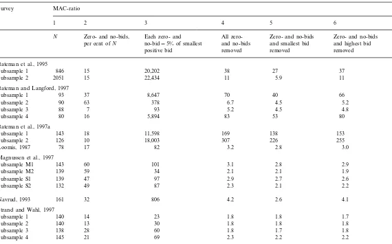
Table 1 reports our empirical results. Column 1 shows the number of observations in each study, while column 2 reports the percentage no- and zero-bids. No- and zero-bids were lumped to-gether in the table because we could not separate them in all surveys. For those studies where more detailed information was available, the proportion of the total sample who refused the payment principle ranged from 6 to almost 14% in the use value studies (Bateman et al., 1995, 1997b) and was over 46% in the study of non-user values (Bateman and Langford, 1997).20
In each case, respondents were asked to state the reasons un-derpinning this response. Analysis of this data showed that (even if we classify those who failed to give such a reason as being ‘protest’ voters) as a proportion of their respective total samples, only between 0.6 and 1.75% of respondents in the use value surveys could be classed as protestors rising to 7% in the non-user survey. These low rates suggest that the surveys were, at least in this respect, successful in that they were considered plausible and credible by respondents.
17Using, for example, 1% of the strictly positive bid yields dramatically higher MAC ratios (see Medin, 1999).
18The assumption that utility is increasing in both income and the public good implies that no respondent has a negative WTP. If in fact some of the no or zero bids reflect negative ‘true’ WTPs, some individuals must have negative marginal utility of either money or the public good. The former is inconsistent with the assumption of equal marginal utility of money, and thus employment of C* as a welfare estimate, while the latter is inconsistent with equal marginal utility of the public good, and thus implies thatC** is not a correct welfare estimate.
19If zero- and no-bids in fact reflect protesters with positive ‘true’ WTPs, using the ‘true’ WTPs in the calculations could have produced either higher or lower MAC ratios than those obtained by omitting zero bids. Roughly, if zero bidders’ ‘true’ WTP values were mainly in the middle range, omission of zero bids would produce too high MAC ratios; if ‘true’ values were very high and/or very low, omission of zero bids would yield too low MAC ratios.
H
.
Medin
et
al
.
/
Ecological
Economics
36
(2001)
397
–
411
Table 1.MACratios (ratio of maximum acceptable costs) under different assumptions on zero- and no-bids and the single highest or lowest bid.21,22(Note that for MACratios B10, values are reported with one decimal)a
Survey MAC-ratio
1 2 3 4 5 6
N Zero- and no-bids, Each zero- and All zero- Zero- and no-bids Zero- and no-bids
and no-bids and highest bid
no-bid=5% of smallest
per cent ofN and smallest bid
removed removed removed
positive bid Bateman et al., 1995
846 15 20,202
Subsample 1 38 27 37
2051 15 22,434 11
Subsample 2 5.9 11
Bateman and Langford, 1997 93
Subsample 1 37 8,647 70 40 66
Subsample 2 90 63 378 6.7 4.5 5.2
88 7 93
Subsample 3 5.2 4.5 4.8
Subsample 4 80 16 5,894 83 53 80
Bateman et al., 1997a
Subsample 1 143 18 11,598 169 138 153
126 10 18,003
Subsample 2 307 226 255
Loomis, 1987 78 17 82 3.2 2.8 3.0
Magnussen et al., 1997 143
Subsample M1 60 101 3.1 2.8 2.9
139 59 34
Subsample M2 2.1 2.1 1.9
Subsample S1 139 47 97 2.9 2.7 2.6
132 49 87 2.3 2.1 2.2
Subsample S2
161 32 806
Navrud, 1993 4.2 2.6 4.1
Strand and Wahl, 1997
140 14 23
Subsample 1 1.8 1.8 1.7
140 13 30 1.8
Subsample 2 1.8 1.8
138 28 60
Subsample 3 1.8 1.7 1.8
145 21
Subsample 4 69 2.3 2.2 2.2
aN,=number of respondents; zero-bids,=respondents reporting a zero WTP; no-bids,=respondents responding ‘no’ to the payment principle question. 21If choice of aggregation unit does not matter, theMACratio=1.
Column 3 reports the first version of the MAC ratios assuming that no- and zero-bids reflect a very small, but positive WTP (5% of the lowest bid in that survey). This yields extremely high MAC ratios, ranging from 23 (subsample 1, Strand and Wahl, 1997) to 22 434 (!) ((subsample 2, Bateman et al., 1995).23Thus, if one accepts the
assumptions underlying the first version of MAC, the estimated aggregate monetary benefit indica-tor is reduced by a facindica-tor of up to about 22 000 by replacing the conventional assumption of equal marginal utility of income by an assumption of equal marginal utility of the environmental good. Column 4 reports the more conservative version of MAC ratios, i.e. afterallzero- and no-bids are omitted from the dataset. This approach yields considerably less extreme MAC ratios varying between approximately 2 (the four subsamples in Strand and Wahl, 1997 and two subsamples from Magnussen et al., 1997) and 307 (subsample 2 in Bateman and Langford, 1997). However, even the smallest MAC ratios of approximately 2 are, in one sense, large, since they imply that using envi-ronmental units as numeraire instead of money almost halves the maximum acceptable per person cost which leaves the project socially desirable. In the study with highest MAC ratio, the maximum acceptable per person cost varies with a factor of up to 307, depending on whether one employs an assumption of, respectively, equal marginal utility of income or of the environmental good.
Table 1 shows that the MAC ratios emerging from the data of Bateman et al. (1995, 1997b) and subsample 1 and 4 in Bateman and Langford (1997) are considerably higher than those of the other surveys. One reason for this might be that these studies contain several very small WTP bids in the sense that the ratio between the smallest and the highest bid reported is large. In subsam-ple 2 from Bateman and Langford (1997), for example, the highest bid reported was £1000, while the lowest strictly positive bid was £0.005. Thus, in this survey, using money as the nu-meraire implies that the net benefits of the person
with the highest WTP is weighted 200 000 times more than the net benefits of the person with the lowest WTP, as compared with the procedure of using environmental units as the numeraire (see Brekke, 1993).
3.4. Sensiti6ity to extreme obser6ations
Column 5 reports MAC ratios when the single
smallest WTP bid is removed from the data, in
addition to removing the zero- and no-bidders. It
turns out that the MAC ratio can be surprisingly sensitive to such removal of one single observa-tion. Particularly interesting is subsample 2 from Bateman et al. (1995) where despite the unusually large sample size of about 1800 observations (af-ter the removal of all zero- and no-bids), the MAC-ratio is almost halved by removing the single smallest strictly positive WTP bid from the data.
To understand this phenomenon, recall the ex-pression for the MAC ratio used in Eq. (15), MAC=(WTP) (WTP−1). Somewhat imprecisely,
one might say that the effect of omitting one observation from the dataset depends on whether this observation’s relative impact on these two averages is very different, or rather, asymmetric. Removing a very small bid may have a large impact on WTP−1, while WTP may be quite
unaffected.24 Removing a high bid, on the other
hand, is likely to affect WTP much more than WTP−1. Column 6 reports MAC ratios when the
single highest WTP bid is removed from the data, in addition to removing the zero- and no-bidders. We see that in the surveys examined here, remov-ing the sremov-ingle highest bid did not affect MAC ratios nearly as much as removing the smallest strictly positive bid.
The above illustrates the importance of obtain-ing accurate information on low WTP bids. To calculate correct MAC ratios, the ability to
distin-24For example, imagine a survey where N=10. Say that nine respondents report a WTP of $10, while one reports $0.05. Omitting the latter observation would change WTP from 9.005 to 10, while WTP−1would change from 2.09 to 0.1. Correspondingly, the MAC ratio would change from 18.8 to 1.
guish between small WTP numbers is essential. It is not obvious that respondents are capable of such fine distinction. Further, existing CV surveys have, of course, not been designed with this prob-lem in mind. One way to alleviate the probprob-lem may be to ask respondents in CV surveys to report their public good requirements in addition to the usual WTP question.25
3.5. Social net benefits
Some of the studies also estimated the costs of the project. For example, in Magnussen et al. (1997) (subsamples S1 and S2), the annual total costs were estimated at between $0.38 and 0.51 million.26 These costs were to be divided between
approximately 8800 households, implying annual costs per household of $43 – 65. The average mon-etary benefit per household (assuming equal mar-ginal utility of income) was estimated at between $111 and 132 per annum. Thus, benefits appeared to substantially exceed costs, and the project was deemed to be socially desirable. Would the policy recommendation of this study be changed if one had, instead, assumed equal marginal utility of the environmental good? If all zero- and no-bids are removed from the dataset, corresponding to the ‘conservative’ MAC ratios reported in column 4, maximum acceptable per household costs (C**) will be between $85 and 97, which is still above the estimated costs; and the project still yields positive social benefits.27 Thus, in this particular
case, the conclusion of the analysis seems robust. Note, however, that since all zero-bids are omitted, many respondents who would most
likely get a negative net benefit have been ex-cluded from the analysis. Thus, both C* andC** may overestimate the projects’ net benefits. Fur-ther, if all no- and zero bids are included, and interpreted as 5% of the lowest strictly positive bid, theC** estimate is reduced to $1.3, which is far less than the estimated annual per household costs, and the conclusion of the cost-benefit analy-sis is changed.
We have also calculated the net social benefits of the projects studied in Loomis (1987), Navrud (1993), Strand and Wahl (1997).28
Estimated net benefits are positive for all these projects when equal marginal utility of income is assumed. If one assumes, instead, equal marginal utility of the public good, net benefits remain positive for the projects in Loomis (1987), Navrud (1993), Strand and Wahl (1997) subsample 1 and 2, provided that no- and zero-bids are removed from the datasets. For Strand and Wahl (1997) subsample 3 and 4, net benefits are negative if a 7% discount rate is assumed, but positive if the discount rate is set to 3.5%. Considering the high MAC ratios, the robustness of the conclusions may be somewhat surprising. Note, however, that when no- and zero-bids are included and counted as 5% of the lowest strictly positive bid, net benefits are nega-tive for all projects.
3.6. Can the results be generalised?
The MAC ratios reported in Table 1 indicate that the way one compares utility between persons may be extremely important in applied cost – benefit analysis. However, the generality of our results depends, of course, on the extent to which the studies we have used are representative of the ‘typical’ response pattern in CVM studies. Also, some of the simplifications employed in our theo-retical model may not hold in practice. One objec-tion is concerned with the fact that our theoretical model assumes onlymarginal changes in the pub-lic good supply, in the sense that any changes in
25A public good requirement question could, for example, be formulated as follows, ‘if a proposed program to increase the salmon population in river X were implemented, you would have to pay $10 per year in increased income taxes. What is thelowestpercentage increase in the salmon popula-tion which would make you willing to pay this cost’?
26We assume the exchange rate between NKR and USD to be 7.828 (31 August, 1998).
27‘Person’ is here used interchangeably with ‘households’, thus, we disregard intra-household conflicts of interest in this example.
individuals’ marginal rates of substitution be-tween the public good and income due to the project can be disregarded. In practice, for many environmental projects, this will not hold for at least some individuals. Regarding the studies mentioned in Table 1, this seems particularly questionable for subsample 1 in Bateman and Langford (1997), and for both subsamples in Bateman et al. (1995).29 However, as mentioned
above, one cannot know a priori whether the calculated MAC ratios will be too high or too low if the public good change is in fact non-marginal, as the errors will generally go in both directions; and in the special case of quasi-linear utility func-tions, Eq. (15) can be used to calculate MAC ratios correctly, even if willingness to pay data does not represent marginal changes.
It is also somewhat difficult intuitively to un-derstand what measuring in ‘environmental units’ really means. Some may dismiss our results on the grounds that the environmental unit has not been well-defined enough in some or all of the studies we have used. All the surveys do consider mea-surement problems and problems related to giving a precise definition of the public good, and all authors appear to have given serious consider-ation to this problem in their survey design. It is certainly often difficult to specify the environmen-tal good in a precise enough way, and this is a problem which all contingent valuation studies have to grapple with. Since the surveys we have used were designed with the income numeraire in mind, questionnaires cannot be expected to have focused on aspects which are considerably more important in our context than in the traditional context. However, since MAC ratios can be ex-pressed using only monetary valuations (see Eq. (15)), respondents do not in practice need to express their valuations using environmental units (i.e. their public good requirements). The issue of defining and understanding what ‘an environmen-tal unit’ means only represents a problem in our context to the extent that misunderstandings re-garding this prevented respondents from actually reporting their true WTPs (in monetary terms). If
the overall pattern of responses in the surveys we have used are typical for CVM surveys, our re-sults on the MAC ratios will also be typical.
4. Conclusions
The results reported above indicate that aggre-gate social benefit estimates may be extremely sensitive to alternative ways of comparing differ-ent individuals’ utility changes. Making non-ve-rifiable assumptions on cardinal and interpersonally comparable aspects of individuals’ utility functions introduces a non-negligible ele-ment of arbitrariness into cost – benefit analysis.
The numerical results are very sensitive to changes in the treatment of extreme WTP obser-vations, in particular no- and zero bids. However, even our most conservative estimates indicate that if one assumes equal marginal utility of the public good for everyone, instead of the usual assump-tion of equal marginal utility of income, aggregate monetary benefit estimates are reduced by a factor of between 2 and 307.
We wish to stress that our aim has not been to argue in favour of one or the other method of making utility interpersonally comparable.
Rather, the lesson from our study is that opera-tionalisation of interpersonal utility comparisons is extremely important for empirical cost – benefit analysis. In the light of this, we believe that cost – benefit practitioners should take on a much more active attitude towards this issue.
One alternative is to take considerably more care when interpreting aggregate social benefit estimates, and emphasise that what one reports in a cost – benefit analysis is not aggregate utility, but aggregate willingness to pay. At the present state of art, we simply do not know whether the two coincide reasonably well.
As a practical approach, Johansson (1998) sug-gests to report costs and benefits in monetary units for subgroups of the population. However, this will only reduce the aggregation problem if one has reasons to believe that the marginal utility of income is similar within each group (Nyborg, 2000). Since marginal utilities are unobservable, such judgements must necessarily be subjective.
Another alternative is to report the number of individuals with positive and negative net benefits, respectively, which would in principle yield the same result as a referendum. This alternative is based on ordinal information only, and does not require particular assumptions on marginal utili-ties. Nor does it require WTP data; a ‘yes’ or ‘no’ would be sufficient. However, the result of such a voting procedure does not necessarily reflect the sign of the change in social welfare. To actually estimate aggregate social benefits, welfare economists must face the question of utility com-parisons explicitly, and address the issue of which methods are actually defensible.
Acknowledgements
We wish to thank John Loomis, Kristin Mag-nussen and Olver Bergland who have kindly pro-vided us with disaggregated data from their own research, and to Kjell Arne Brekke and Rolf Aaberge for comments.
References
Arrow, K.J., 1951. Social Choice and Individual Values. Wi-ley, New York.
Bateman, I.J., Langford, I.H., 1997. Budget-constraint, tempo-ral and question-ordering effects in contingent valuation studies. Environ. Planning A 29 (7), 1215 – 1228.
Bateman, I.J., Langford, I.H., Turner, R.K., Willis, K.G., Garrod, G.D., 1995. Elicitation and truncation effects on contingent valuation studies. Ecol. Econ. 12 (2), 161 – 179. Bateman, I.J., Munro, A., Rhodes, B., Starmer, C., Sugden, R., 1997a. A test of the theory of reference dependent preferences. Q. J. Econ. 112 (2), 479 – 505.
Bateman, I.J., Langford I.H., McDonald, A.L., Turner, R.K., 1997b. Valuation of the recreational benefits of a proposed sea defence scheme at Caister, East Anglia: a contingent valuation study. Report to Sir William Halcrow and Part-ners of Great Yarmouth Borough Council, School of Environmental Sciences, University of East Anglia, p. 165. Brekke, K.A., 1993. Does Cost – Benefit Analyses Favour En-vironmentalists? Discussion Paper 84. Statistics Norway, Oslo.
Brekke, K.A., 1997. The numeraire matters in cost – benefit analysis. J. Public Econ. 64, 117 – 123.
Bromley, D.W., 1990. The ideology of efficiency: searching for a theory of policy analysis. J. Environ. Econ. Manage. 19, 86 – 107.
Broome, J., 1992. Counting the Cost of Global Warming. White Horse Press, Cambridge, UK.
Carson, R.T., 1999. Contingent Valuation: A User’s Guide. Manuscript, Department of Economics, University of Cali-fornia, San Diego.
Dre´ze, J., 1998. Distribution matters in cost – benefit analysis. J. Public Econ. 70, 485 – 488.
Dre`ze, J., Stern, N., 1987. The theory of cost – benefit analysis. In: Auerbach, A.J., Feldstein, M. (Eds.), Handbook of Public Economics, vol. 2. Elsevier (North-Holland), Am-sterdam, pp. 909 – 990.
Frisch, R., 1932. New Methods of Measuring Marginal Util-ity, Beitra¨ge zur O8konomischen Theorie 3. Mohr, Tu¨bingen.
Hammond, P.J., 1979. Straightforward individual incentive compatibility in large economies. Rev. Econ. Studies 46, 263 – 282.
Hammond, P.J., 1990. Theoretical progress in public econom-ics: a provocative assessment. Oxford Econ. Pap. 42, 6 – 33. Hammond, P.J., 1994. Money metric measures of individual and social welfare allowing for environmental externalities. In: Eichhorn, W. (Ed.), Models and Measurement of Wel-fare and Inequality. Springer, Berlin.
Harsanyi, J.C., 1955. Cardinal welfare, individualistic ethics, and interpersonal comparisons of utility. J. Political Econ. 63 (4), 309 – 321.
Hicks, J., 1939. The foundations of welfare economics. Econ. J. 49, 696 – 712.
Johansson, P.-O., 1998. Does the choice of numeraire matter in cost – benefit analysis. J. Public Econ. 70, 489 – 493. Kelman, S., 1981. Cost – Benefit Analysis. An Ethical Critique,
Regulation, pp. 33 – 40.
Little, I.M.D., Mirrlees, J.A., 1994. The costs and benefits of analysis: project appraisal and planning twenty years on. In: Layard, R., Glaister, S. (Eds.), Cost – Benefit Analysis, second ed. Cambridge University Press, Cambridge, pp. 199 – 231.
Loomis, J., 1987. Balancing public trust resources of Mono Lake and Los Angeles’ water right: an economic approach. Wat. Resour. Res. 23 (8), 1449 – 1456.
Magnussen, K., Rymoen, E., Bergland, O., Bratli, J.L., 1997. Miljøma˚l for vannforekomstene, SFT-rapport 97:36. State Pollution Agency, Oslo (in Norwegian).
Medin, H., 1999. Betydning av ma˚leenhet i verdsetting av miljøgoder. Empiriske eksempler, Reports 99/9. Statistics Norway, Oslo (in Norwegian).
Medin, H., Nyborg, K., Bateman, I., 1998. The assumption of equal marginal utility of income: how much does it matter? Discussion Paper 241. Statistics Norway, Oslo (available at http://www.ssb.no).
Navrud, S., 1993. Samfunnsøkonomisk lønnsomhet av a˚ kalke Audna, Utredning for Direktoratet for naturforvaltning nr. 1993 – 1994 (in Norwegian).
Sen, A.K., 1977. Rational fools: a critique of the be-havioural foundations of economic theory. Phil. Public Affairs 6, 317 – 344.
Sen, A.K., Williams, B. (Eds.), 1982. Utilitarianism and Be-yond. Cambridge University Press, Cambridge.
Strand, J., 1985. Verdsetting av reduserte luftforurensninger fra biler i Norge. Memorandum no. 1. Department of Economics, University of Oslo (in Norwegian).
Strand, J., Wahl, T.S., 1997. Verdsetting av kommunale friomra˚der i Oslo. SNF-report no. 82/97. Centre for
Ap-plied Research, Oslo (in Norwegian).
Unsworth, R.E., Bishop, R.C., 1994. Assessing natural re-source damages using environmental annuities. Ecol. Econ. 11, 35 – 41.
van Praag, B.M.S., 1991. Ordinal and cardinal utility. An integration of the two dimensions of the welfare concept. J. Econometr. 50, 69 – 89.
Vatn, A., Bromley, D.W., 1994. Choices without prices without apologies. J. Environ. Econ. Manage. 26, 129 – 148.