Production and preventive maintenance rates control for
a manufacturing system: An experimental design approach
A. Gharbi
*
, J.P. Kenne
University of Que&bec, E!cole de Technologie Supe&rieure, Production Systems Design and Control Laboratory, Department of Automated Production Engineering, 1100, Notre Dame Ouest, Montre&al, Que., Canada H3C 1K3
Received 26 September 1998; accepted 5 April 1999 Abstract
In this paper, a multiple-identical-machine manufacturing system with random breakdowns, repairs and preventive maintenance activities is considered. The objective of the control problem is to"nd the production and the preventive maintenance rates of the machines so as to minimize the total cost of inventory/backlog. By combining analytical formalism and simulation based statistical tools such as experimental design and response surface methodology (RSM), an approximation of the optimal control policy is obtained. A numerical example is presented to illustrate the usefulness of the proposed approach. It is found that the complexity of the experimental design problem remains constant (33 factorial design) when the number of machines increases. Based on the obtained results, the extension of the proposed approach to more complex manufacturing systems is discussed. ( 2000 Elsevier Science B.V. All rights reserved.
Keywords: Preventive maintenance; Production control; Stochastic dynamic programming; Simulation; Experimental design; RSM
1. Introduction
The production planning problem for manufac-turing systems, which is subject to uncertainties such as demand#uctuations, machine failures, etc., has attracted the attention of numerous re-searchers. During the past 15 years, a number of methods have been reported for determining eco-nomic quantities for di!erent products on a single or multiple machines. The spirit of the classical approaches is more in keeping with the pioneering
*Corresponding author. Tel.:#1-514-396-8969; fax: #1-514-396-8595.
E-mail address:[email protected] (A. Gharbi)
work of Kimemia and Gershwin [1] in which the system uncertainties have been modeled by homo-geneous"nite state Markov processes. This line of work has been continued by Akella and Kumar [2] and Sharifnia [3]. The approach has been extended by Boukas and Yang [4] who consider the fact that the machine failure depends also on its age. The related age dependent set of dynamic programming equations was solved numerically for a two-ma-chine, one-product system. However, considering the numerical scheme presented in Boukas and Yang [4], it becomes di$cult to obtain the optimal control for a large-scale manufacturing systems. A way to cope with this di$culty is to develop heuristic methods which are based on the size reduction of the considered control problem. Di!erent approaches have been proposed in the
literature to derive simple near-optimal control policies of manufacturing systems.
The concept of hedging point policy, introduced by Kimemia and Gershwin [1], is one of the simplest ways of"nding near-optimal control pol-icies for manufacturing systems. More precisely, such a policy suggests that when the machine is up, one should produce at the maximum possible rate when the inventory level is less than a given thre-shold, produce on the demand ratedif the inven-tory level is exactly equal to the threshold, and not produce at all if the inventory level exceeds the threshold. Further details on the concept of hedg-ing point policy can be found in Akella and Kumar [2]. In addition, a modi"ed version of such a policy, namely age-dependent hedging point policy is pre-sented in Kenne and Gharbi [5].
Another approach is to develop a hierarchical control method using singular perturbation methods such as in Lehoczky et al. [6], Sethi et al. [7] and Kenne [8]. However, including the age-dependent failure rates of machines, the application of such approaches becomes very complex. This is due to the fact that although machines are initially identical, they have obviously di!erent dynamics while producing.
In this paper, we propose an alternative ap-proach which consists of developing an optimiza-tion procedure to obtain the response surface model of the cost incurred in terms of parameters of a near-optimal control policy. The procedure is based on a series of simulation experiments and combines advantages of both analytical and simu-lation based models. Comparing this methodology with the `optimum numerical grid founding methodapresented by Kenne et al. [9], this paper proposal is extracted from small number of simula-tion runs meanwhile its model includes signi"cant main factors and interactions. The same approach was recently used by OG mer and Serpil [10] to explicitly examine the performance of a multi-item, multi-line, multi-stage JIT system under di!erent factors settings. We studied the problem for a multiple-identical-machine, one-product manufac-turing system considering machine-age-dependent down times. Further details on the concepts of experimental design and/or response surface meth-odology (RSM), used hereinafter, can be found in
Kenne and Gharbi [5], Gharbi and Kenne [11] and Abdulnour et al. [12].
Optimization equations of the analytical model have generally a complex structure, and in the case of non-homogeneous processes, there is no explicit functional relationship between the performance criteria (i.e., incurred cost) and the independent variables of the model (i.e., stock and machines ages). In this paper a useful procedure which com-bines both the analytical control approach and the experimental design method is presented. De"ning the control variables as parameters of a modi"ed hedging point policy, which are also machine age dependent, their best values are given by minimiz-ing the estimated relationship between the cost and these variables. Thus, the aim of the proposed ap-proach is to provide the best values of the de"ned parameters in order to improve the control policies. These parameters are: (i) the stock level of"nished goods, (ii) the oldest machine age at which it is necessary to send it to preventive maintenance, (iii) the oldest machine age under which a null stock level is needed.
The paper is organized as follows. In Section 2, we present the notation and the problem statement of the considered production planning problem. The properties of the value function and also the best approximation of the optimal control policy for suitable values of parameters are given in Sec-tion 3. The control approach and the simulaSec-tion model are demonstrated respectively in Sections 4 and 5. The experimental design and response surface methodology are included in Section 6 while Section 7 concludes the paper.
2. Notation and problem statement
In this paper, we shall as far as possible use the notation summarized as follows:
m number of machines f
i(t) stochastic capacity process of the machinei, 1)i)m
jiab()) transition rates from modesatobrelated to the machinei, 1)i)m
u(t) production rate of the system
u(t) vector of machines preventive mainten-ance rates
u(t) control policy vector ;
. maximal production rate of a machine B maximal preventive maintenance rate of
a machine
k(t) capacity process of the system (number of operational machines)
K(a) set of admissible controls at modea
G(a, )) instantaneous cost at modea
J()) expected and discounted cost function
v()) value function
X inventory threshold level parameter
A switching machine age parameter related to the production policy
B preventive maintenance age parameter Cost estimated cost function
The system under study consists of m identical machines producing one part type. The operational mode of the machine i can be described by a stochastic process f
i(t) (1)i)m). Such a
ma-chine is available when it is operational (fi(t)"1) and unavailable when it is under repair (fi(t)"2) or under preventive maintenance (fi(t)"3). The stochastic process has then three states,f
i(t)3Bi"
M1, 2, 3N, which can be described statistically by the following state probabilities:
The transition rate from state 1 to state 2, for each machinei, is represented byji12(.)"/(a
i) and
the function/(.) express the age dependance of the failure rate of the machine i. The transition rate from state 1 to 3 is assumed to be a control variable. Letji13())"ui()) whereu~1i ()) represents the ex-pected delay between the call for a technician and his arrival as de"ned in Boukas and Yang [4]. We
assume that transition ratesji21andji31are given constants.
Letk(t) be the"nite state machine capacity pro-cess of the system. Here k(t)3M"M0, 1,2,mN represents the number of machines available for production at time t. This process is modeled by a continuous time Markov chain de"ned on MX,F,PN with in"nitesimal operator Q(a,u), where a"(a
1,2,am) and u"(u1,2,um) are
vector of ages and vector of preventive main-tenance rates respectively. Here Q(.)"Mq
ij(.)N is
Such a process is a birth}death process.
The system behavior is described by a hybrid state which comprises both a discrete and a tinuous component. The discrete component con-sists of the discrete event stochastic processk(t) and the continuous component consists of continuous variablesx(t) anda
i(t) (i"1,2,m). These variables
correspond to the inventory/backlog of the product and the cumulative age of the machinei respective-ly. Letu(t)3Rbe the production process fort*0. The state variables, namely inventory/backlog and machines ages, are described by the following dif-ferential equations:
x5(t)"u(t)!d, x(0)"x, (3)
a5(t)"f(u(t)), a(0)"a, (4)
where;
.andBare given maximal production and preventive maintenance rates of an individual ma-chine respectively. Our decision variables are the production rate and preventive maintenance rates over time andK(a) is the set of admissible decisions at the modea. By controllingu()), one decreases the machines failure frequencies and hence im-proves the system availability. LetG(a,a,x,u,u) be the cost rate de"ned as follows:
G(a,a,x,u,u)"c`x`#c~x~#ca, ∀a3M, (6)
wherec`andc~are respectively, cost incurred per unit produced part for positive inventory and back-log, x`"max(0,x(t)), x~"max(!x(t), 0). The constantcais used to penalize the repair and pre-ventive maintenance activities and is de"ned as follows:
Our objective is to control the production rateu(t) and the preventive maintenance rateu(t) to minimize the expected discounted cost given by
J(a,x,u)"E
GP
=0
e~otG(k(t),x,u)dtDx(0)"x,
a(0)"a,k(0)"a
H
(8) subject to constrains given by Eqs. (1)}(6). The value function of such a problem isv(a,x)" inf
u|K(a)
J(a,a,u) ∀a3M. (9)
A su$cient condition for optimal control states that the value function given by (9) satis"es the following Hamilton}Jacobi}Bellman (HJB) equa-tions: optimality conditions given by (10) and elementary properties of the value function can be found in Kenne [8] and Boukas and Kenne [13].
The optimal control policy (uH()),uH())) denotes a minimizer overK(a) of the right-hand side of Eq. (10). This policy corresponds to the value function described previously. Then, when the value func-tion is available, an optimal control policy can be obtained from Eq. (10). Some authors [4] used numerical approaches, restricted to small size sys-tems (for example a one or two machines manufac-turing system producing one part type) to show that the hedging point policy remains valid and it depends on the age of the machine. It is now well known that the analytical solution of Eqs. (10) for obtaining the value function and the related opti-mal control policy, is almost impossible. Instead of solving Eq. (10), either analytically or numerically, we propose an alternative solution which is based on the heuristic control policy presented in the next section.
3. Heuristic control policy
3.1. Multiple and non-identical machines systems
The modi"ed hedging point policy, presented later, is described by the following parameters:
X The value of the threshold or number of parts to maintain in stock to hedge against machines breakdowns.
A
i The age of the machinesary to stock parts. Before this age, the ma-i, at which it is
neces-chineiis assumed to be new, and a production at the demand rate is suggested if the other machines are new.
B
i The age at which the machinepreventive maintenance when the thresholdi is sent to
value X is achieved. In such a situation, the machine will be sent to preventive maintenance randomly. There is a random delay (given by a random distribution with mean equal to 1/B) from the machine age B
i to the maintenance
time.
With these parameters, the proposed control policy states the following:
1. Preventive maintenance policy:The maintenance rate ui()) can be described by the following
2. Production control policy: The production rate
u()) can be described by the following machine-age-dependent policy:
With this parameterized control policy (depending onA
i,BiandX),i"1,2,m, the best
approxima-tion ofv(a,x), given by (9), is found for some values of A
i, Bi and X. Simulation experiments and
re-sponse surface methodology are the sources used to approximate the relationship between v(a,x) and
A
i,Bi,X. It is from this estimated function that the
corresponding optimum values (AH
i,BHi,XH) are
obtained. This leads to a 2m#1 factor problem. For example, one has a 3, 5 or 7 factor experimental design problem for a one, two or three machine manufacturing system respectively. The experi-mental design problem with 2m#1 factors, each one having three levels, becomes di$cult to solve for largem. A 32m`1factorial experimental design is selected to consider the convexity property of the value function. That property is established in Kenne [8]. With a large number of experiments (i.e., 32m`1), the 32m`1~pfractional factorial designs, with
p(2m#1, are potentially desirable but they are not generally recommended designs. The main rea-son is that such designs have alias relationships that involve the partial aliasing of two-degrees-of-free-dom components of interaction. This, in turn, results in a design that will be di$cult if not impossible to interpret if interactions are not negligible [14].
3.2. Multiple and identical machines systems
With identical machines, the parametersA
iand
B
i of the previous policy are replaced by A and
Bde"ned as follows:
A The age of the oldest machine at which it is necessary to stock parts. Before this age, the machines are assumed to be in new condition and a production at the demand rate is sugges-ted.
B The age of the oldest machine at which one can plan to send it to preventive maintenance when the threshold is achieved. The oldest machine is then sent to preventive maintenance randomly.
With these parameters, the modi"ed control policy implies the following:
1. Preventive maintenance policy:The maintenance rate u
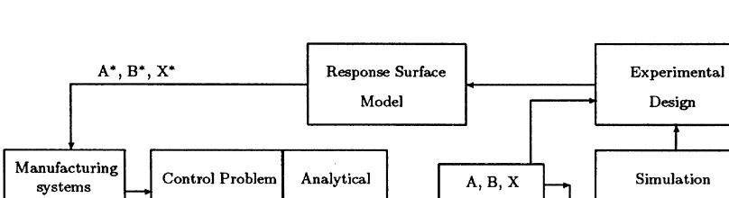
Fig. 1. Structure of the proposed control approach.
1. C if max(a(t) ))B for all i3M1,2,mN then u
k())"0 where k refers to the oldest ma-chine;
1. C if max(a(t))'Bthenu
i()) is given by Eq. (11). 2. Production control policy: The production rate
u(.) can be described by the following machine age-dependent policy:
1. C if max(a(t)))Athenu(.,a) is given by Eq. (12);
1. C if max(a(t))'Athenu(.,a) is given by Eq. (13).
Let us now present the control approach used to generate the best values of input factorsA,BandX.
4. Control approach
The results from traditional methods of planning in the environment of the manufacturing system are not su$cient to reach a comfortable level of desired performances. To improve these methods, we aug-ment the descriptive capacities of conventional simulation model by using both analytical and simulation based statistical analysis. The resulted structure is depicted in Fig. 1.
The problem of the optimal#ow control for the considered manufacturing system is described in the blockManufacturing system(uH(.)"?). The ob-jective in this block is to"nd the best parameters of the control variable u(.), called production and maintenance rates (i.e.,A,BandX) which improves the related output (i.e., the incurred cost). The aim of theControl Problem Formulationblock (Fig. 1) is to develop a mathematical representation of the system based on some simpli"ed hypothesis. By applying an Analytical Approach, such as in
Lehoczky et al. [6], the structure of a feedback control policy is derived. Such a policy is para-meterized by the factors A, B and X and is con-sidered as an input of the Simulation model. The cost related to each entry, given by values of input factors, is de"ned as the output of theSimulation model.
TheExperimental designblock determines from
values of the input factors and the related cost values, the input factors and/or their interactions which have signi"cant e!ects on the output. These factors or interactions are then considered as the input of theResponse surface model, to"t the rela-tionship between the cost and the input factors. From this estimated relation, the optimal values of the input factors, called AH,BH and XH, are determined. The related hedging point policy
u(AH,BH,XH) is then an improved age dependent hedging point policy to be applied to the manufac-turing system.
The application of the structure, depicted in Fig. 1, to the production and maintenance rates planning of the system under study is presented in the next sections. A set of hedging point policies are implemented in the simulation model, described in Section 5, by varying the input factors.
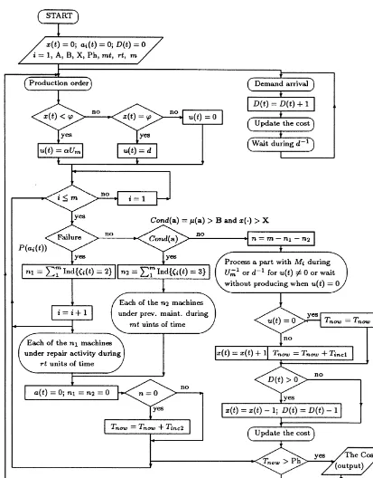
5. Simulation model
the system occurs at discrete instants in time in accordance with prede"ned operating rules. Due to the fact that the experimental conditions are fully known, controllable and reproducible (i.e., for the hedging point policy and given values ofA,Band
X), without loosing the generality of the approach we adopt the network structure model. The net-work pictorially represents the system of interest by a set of symbols (nodes and branches) interfaced with user written subroutines if necessary.
Our process consists of a time-ordered sequence of events combined with several nodes, activities and oriented branches. The proposed simulation model consists of several networks; each of them describes a speci"c contribution in the system modeling purpose (i.e., demand generation, control policy generation, states of the machine, inventory control, etc.). The diagram of the proposed simula-tion model is depicted in Fig. 2 with the following notations:
f Control policy: The production control policy
given by (11)}(13) is modeled by usinguandk(.) de"ned by
ability distribution of the machine i which is assumed to be given by:
P(a
i(t))"1!exp(!k1aki2(t)) (16)
where k1 and k2 are given constants and the machine agea
i(t) is de"ned here as the number of
produced parts since the last intervention on the machine (repair or preventive maintenance). An increasing failure rate (IFR) is given by (16) with
k
1@1 andk2*4. One can then obtain the
well-known IFR such as Weibull distribution with suitable values ofk
1andk2and design the
ap-propriate preventive maintenance controllers. For further information on the IFR, we refer the reader to Sheng-Tsaing [16] where both Weibull
and extreme-value distributions were used to enhance the reliability of a given process. The repair and maintenance time are represented by rt and mt respectively.
f Inventory control: D(t), Ph and¹
/08 denote, re-spectively, the cumulative demand, the produc-tion horizon and the current simulaproduc-tion time. The increments of ¹
/08, namely ¹*/#1 and
¹
*/#2are given by the following expressions:
¹
rt if the repair was performed,
mt otherwise, (18)
for a given ¹
n which corresponds to the
in-crement of the simulation time.
A detailed simulation model is developed using SLAM II1 and FORTRAN subroutines [15,10] which integrates the modi"ed hedging point policy providing an output for each given (A,B,X). How-ever, the basic idea of such a model can be found in Kenne et al. [9] or in Gharbi and Kenne [11] for the sake of completeness.
In order to obtain the cost (output) correspond-ing to each entry (i.e., input factorsA,BandX) the behavior of the system has been simulated using the above diagram (Fig. 2) in the case ofm"4 (i.e., four machines manufacturing system). A large value was assigned to Ph to be sure that the "nite horizon cost related to that Ph corresponds to the steady state. Some simulation experiments were done to achieve the steady state. With Ph"7000, the obtained cost per unit of time is not time depen-dent. Next, four simulation replications are con-sidered for each entry with di!erent values of the stream number. Such a number is used to generate di!erent values for a random variable for di!erent simulation experiments. The simulation data is summarized as follows: d"0.75, ;
."0.25,
c`"1, c~"10, q~131"2, k
1"0.001, k2"4 and
q~121"10. The procedure of varying simultaneously
A,BandX, called experimental design, is presented in the next section.
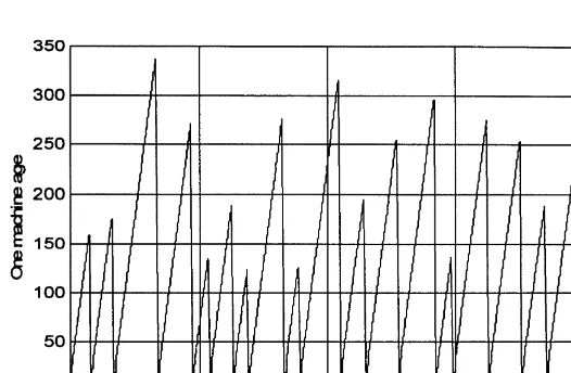
Fig. 3. One machine age trajectory (number of produced part vs. time).
6. Experimental design and response surface methodology
The objectives of this section are: (i) to determine if the input parameters a!ect the response, (ii) to estimate the relationship between the cost and signi"cant factors and "nally (iii) to compute the optimal values of estimated factors.
6.1. Experimental design
Generally, the studies based on the optimal pro-duction control problem of manufacturing systems use generally the cost of producing parts as criteria index function. The speci"c form of this function depends on the problem statement. Here, we collect and analyze data for a steady-state cost which approximates the cost de"ned by Eq. (8) as close as possible. The experimental design is concerned with (i) selecting a set of input variables (i.e., factors
A,BandX) for the simulation model; (ii) setting the levels of selected factors of the model and deciding on the conditions, such as length of runs and num-ber of replications, under which the model will be run.
In this paper, we assume that input factors (A,BandX) are present at three levels due to the convexity of the value function (we are concerned about curvation of the response surface). Hence, the response surface, described by a second-order
model requires that at least three levels of design parameters be studied, so that the coe$cient in the model can be estimated [17]. Therefore, 3nfactorial experimental design is necessary. The levels of the factors should be chosen carefully so that they represent the domain of interest. The levels of X,
A and B are chosen from the observation of the machine-age trajectory and output given by some preliminary runs made o!-line.
Fig. 3 shows that, from the initial time to the"rst jump time (when a breakdown occurs) a machine age increases from zero to 155 parts. The machine age is then set to zero following the repair. When the machine is repaired, it again produces parts and its age increases until 175 where a second break-downs occurs. After it has been repaired, the ma-chine is up again and a behavior similar to the previous ones is performed. Such behaviors take place until time"2000. For this period, the mean age at which failures occur is 195 parts. Intuitively, the preventive maintenance must be done around this age for an optimal control policy. This obser-vation is useful to judiciously choose levels of factors A and B to conduct the experimental design.
Table 1
Levels of the independent variables
Factor Low level Center High level Description
B 0 160 320 Preventive maintenance variable
A 20 50 80 Inventory policy variable
X 0 8 16 Stock level variable
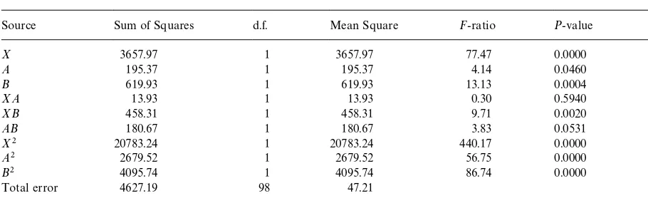
Table 2 ANOVA table
Source Sum of Squares d.f. Mean Square F-ratio P-value
X 3657.97 1 3657.97 77.47 0.0000 S
A 195.37 1 195.37 4.14 0.0460 S
B 619.93 1 619.93 13.13 0.0004 S
XA 13.93 1 13.93 0.30 0.5940 NS
XB 458.31 1 458.31 9.71 0.0020 S
AB 180.67 1 180.67 3.83 0.0531 NS
X2 20783.24 1 20783.24 440.17 0.0000 S
A2 2679.52 1 2679.52 56.75 0.0000 S
B2 4095.74 1 4095.74 86.74 0.0000 S
Total error 4627.19 98 47.21
Total 107 R-squared"0.88
Let us now decide on the nature of simulation runs as well as the number of replications. The steady state of the cost is achieved after the simula-tion of the model during a period of 7000 time units. Owing to the stochastic nature of the produc-tion process, this value can be di!erent for two runs with the same input variables. Some pilot simula-tion runs were done in order to estimate the num-ber of replications needed to access the variability of the output analysis. We then selected four repli-cations; therefore 108 (27]4) simulation runs were made. Runs used randomly assigned treatments by choosing di!erent stream numbers for each replica-tion. All possible combinations of di!erent levels of factors are provided by the response surface design considered herein. This design is used to study and understand the e!ects that some parameters, namely A, B and X have on the performance measure (i.e., the cost).
The statistical analysis of the simulated data con-sists of the multi-factor analysis of the variance
(ANOVA). This is done by using a statistical soft-ware, such as STATGRAPHICS, to provide the e!ects of the three independent variables on the dependent variable. Table 2 illustrates a particular ANOVA, especially designed for RSM [18], which corresponds to the generated data. For each main e!ect, interaction and quadratic e!ect, Table 2 in-cludes the Sum of Squares, the degree of freedom (d.f.), the Mean Square, anF-ratio, computed using the residual mean square, and the signi"cance level of the P-value. Table 2 also includes the Sum of Squares, the d.f. and the Mean Square of the residual.
From Table 2, we see that the main factorsX,
Aand Bare signi"cant (symbol S in the last col-umn) for the dependent variable at 0.05 level of signi"cance. This indicates that di!erent values of the independent variables X, A and B result in di!erent performance values for the dependent variable. The interaction XB is also signi"cant
ABare not. A signi"cant interaction implies that, if possible, an appropriate combination of indepen-dent variables should be selected in such a way that the performance criteria (i.e., the cost) is minimized.
The ANOVA table also shows that all quadratic e!ects are signi"cant at 0.05 level of signi"cance which indicates that the input factor levels a!ect the output. It is important to note thatX2 signi"-cantly a!ects the response. This con"rms the quad-ratic approximation form on the stock, related to the cost function, made by some authors in the control literature [19] without the concept of ma-chine-age-dependent failure rates. The third-order interaction (ABX) was neglected or added to the error. This assumption is supported by the stepwise analysis (as in the STATGRAPHICS software) which provide very small coe$cients for such inter-actions or e!ects related to the response surface model.
The R-squared value of 0.88, presented in Table 2, states that about 90% of the total variabil-ity is explained by the model [20]. The obtained model includes three main factors (X,AandB), one interaction (BX) and three quadratic e!ects (A2,
B2 and X2). In the next section, we explore the RSM approach to estimate the relation between the Cost and signi"cant e!ects.
6.2. Response surface methodoloy
Response surface methodoloy is a collection of mathematical and statistical techniques that are useful for modelling and analyzing problems in which a response of interest is in#uenced by several variables and the objective is to optimize this re-sponse [14]. We assume here that there exists a function/ofA,BandXthat provides the value of the cost corresponding to any given combination of factors levels. That is
Cost"/(A,B,X). (19)
The function/(.) is called the response surface and is assumed to be a continuous function ofA,Band
X. Due to the convexity property of the value function associated to (8), the "rst-order response surface model is rejected. We choose the
second-order model given by
Cost"b0#+k
a random error. The number of distinct design points (or simulation runs) must be at least
p"1
2(k#1) (k#2)"10, sincepis the number of
terms in the model in (20). More details on this condition and others features on response surface can be found in Khuri [21]. The basic idea of the development presented in this section is given in Khuri [21]. Here, we provide the details in this particular case (k"3).
From STATGRAPHICS, the estimation of b is performed and the following seven coe$cients achieved:b0"113.87,b1"!1.277,b2"!0.221, b3"!9.097, b23"2.621]10~3, b11"0.0117, b22"5.085]10~4, b33"0.523. In Section 6.1, two e!ects was proved to be unimportant and the corresponding response surface coe$cients are null (no signi"cant information can be detected from the related entry). The cost function is then given by
Cost"b0#b1A#b2B#b3X#b11A2
#b
22B2#b33X2#b23BX. (21)
The near-optimal age-dependent hedging point policy to be applied to the considered manufactur-ing system is de"ned by A"55, B"197 and
X"8. These values are determined using a numer-ical grid founding optimal method.
6.3. Results analysis and extensions
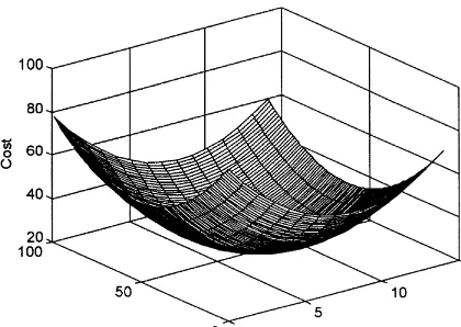
Fig. 4. Response surface of the cost (AH"55, BH"197, XH"8)
Given that the near-optimal control policy, given by Eqs. (11)}(13), is still valid for allm'0 (number of identical machines), one can concludes that:`A control problem in anmmultiple identical machin-es system, under the proposed approach is equiva-lent to a 33factorial experimental design problem related to the control policy (11)}(13)a.
With these results, one can resort to additional aspects such as stochastic demand, multiple prod-ucts, etc. in order to control more complex manu-facturing systems. It is well known that such a problem is very di$cult to solve through the classical approaches such as those based on HJB equations, which need restrictive hypotheses to be tractable. In the proposed approach, the simulation model takes into account those aspects and give the corresponding output. These aspects will a!ect the ANOVA table and the corresponding response sur-face model. An expression similar to (21) will then give the optimum values of parameters X, A and
Bthrough the response surface methodology. How-ever,"nding near-optimal control for systems with machines in tandem remains an open question in the literature and is the next step of our main research objective.
7. Conclusion
A production control approach for manufactur-ing systems, based on simulation experiment is pre-sented. We investigated the near-optimal control
policy of a non-homogeneous Markov process, for which the concept of hedging point policy is still valid under some speci"cations. These speci" ca-tions consist of parameters called in this paper the independent variables. A simulation model has been developed to describe the dynamic production problem using the machine-age-dependent hedging point policy. Then an experimental design was used to investigate the e!ects of speci"ed factors on the cost incurred during the production horizon. The 33 factorial design was selected to identify the complication and to solve the analytical control problem.
The proposed approach combines simulation and statistical analysis to provide the estimation of the cost function related to the considered control problem. A RSM was used to perform this function in terms of signi"cant main factors and interactions given by the experimental approach. From the estimation of the cost function, the best values of control parameters have been computed. It is quite clear that this approach can also be applied to a system with stochastic demand and multiple products. Although, it has not been proven that the hedging point policy is still optimal for such a system, the proposed methodology can be used for obtaining a near-optimal control policy using the concept of machine-age hedging point policy.
References
[1] J.G. Kimemia, S.B. Gershwin, An algorithm for computer control of production in#exible manufacturing systems, IIE Transactions 15 (1983) 353}362.
[2] R. Akella, P.R. Kumar, Optimal control of production rate in a failure prone manufacturing system, IEEE Transac-tions on Automatic Control 31 (2) (1986) 116}126. [3] A. Sharifnia, Production control of manufacturing system
with multiple machine state, IEEE Transactions on Auto-matic Control 33 (7) (1998) 620}625.
[4] E.K. Boukas, H. Yang, Manufacturing#ow control and preventive maintenance: A stochastic control approach, IEEE Transactions on Automatic Control 41 (6) (1996) 881}885.
[6] J. Lehoczky, S. Sethi, H.M. Soner, M. Taksar, An asymp-totic analysis of hierarchical control of manufacturing systems under uncertainty, Mathematics of Operations Research 16 (3) (1991) 596}608.
[7] S. Sethi, Y. Houmin, Q. Zhang, X.Y. Zhou, Feedback production planning in a stochastic two-machine# ow-shop: Asymptotic analysis and computational results, International Journal of Production Economics 30}31 (1993) 79}93.
[8] J.P. Kenne, Plani"cation de la Production et de la Main-tenance des Syste`mes de Production: Approche HieH rar-chiseHe, Ph.D Thesis, EDcole Polytechnique de MontreHal, UnversiteH de MontreHal, 1997.
[9] J.P. Kenne, A. Gharbi, E.K. Boukas, Control policy simu-lation based on machine age in a failure prone one-ma-chine, one-product manufacturing system, International Journal of Production Research 35 (5) (1997) 1431}1445. [10] F.B. OGmer, E. Serpil, Simulation modelling and analysis of a JIT production system, International Journal of Produc-tion Economics 55 (1998) 203}212.
[11] A. Gharbi, J.P. Kenne, Production rate control and design problem in a failure prone manufacturing system, Pro-ceedings of the 6th Industrial Engineering Research Con-ference, Miami, USA, 1997, pp. 813}819.
[12] G. Abdulnour, R.A. Dudek, M.L. Smith, E!ect of maintenance policies on just-in-time production system,
International Journal of Production Research 33 (1995) 565}583.
[13] E.K. Boukas, J.P. Kenne, Maintenance and production control of manufacturing systems with setups. Lectures in Applied Mathematics (1997) 55}70.
[14] D.C. Montgomery, Design and Analysis of Experiments, fourth ed., Wiley, New York, 1997.
[15] A.B. Pritsker, Introduction to Simulation and SLAM II, third ed. Systems Publishing Corporation, West Lafayette, IN, 1986.
[16] T. Sheng-Tsaing, Optimal preventive maintenance policy for deterioring production systems, IIE Transactions 28 (1996) 687}694.
[17] J.A. Cornell, How to Apply Response Surface Method-oloy, American Society for Quality Control Press, Mil-waukee, WI, 1990.
[18] G.E. Box, N.R. Draper, in: Empirical Model Building and Response Surfaces, Wiley, New York, 1987.
[19] S.B. Gershwin, Manufacturing Systems Engineering, PTR Prentice Hall, Englewood Cli!s, NJ, 1994.
[20] R.A. Johnson, D.W. Wichern, Applied Multivariate Stat-istical Analysis, third ed., Prentice Hall, Englewood Cli!s, NJ, 1992.