*Corresponding author. Tel.:#49-431-880-4581; fax: #49-431-880-1531.
E-mail address:[email protected]}kiel.de (R. Kolisch).
Integration of assembly and fabrication for
make-to-order production
R. Kolisch*
Fachgebiet Baubetriebswirtschaftslehre, Institut fu(r Betriebswirtschaftslehre, Technische Universita(t Darmstadt, Hochschulestr. 1, 64289 Darmstadt, Germany
Received 27 April 1998; accepted 4 February 1999
Abstract
The problem of make-to-order production is as follows. A number of customer-speci"c orders have to be assembled in a multi-project type environment. Each order is made of di!erent assembly jobs which are interrelated by precedence constraints. To be processed, an assembly job requires in-house fabricated and out-house procured parts as well as capacity of assembly resources (assembly workers, power tools). Di!erent customer orders need the same part types and hence the fabrication of parts has to take into account lot sizing decisions. The overall problem is how to coordinate fabrication and assembly with respect to scarce capacities in the assembly and the fabrication such that the holding- and setup-cost of the entire supply chain}fabrication}assembly}are minimized. This problem has not been treated in the literature so far. Hence, we give a mixed}integer programming model for the problem and discuss its properties. Afterwards, we propose a simple, two-level backward oriented heuristic and evaluate it on a set of benchmark instances. ( 2000 Elsevier Science B.V. All rights reserved.
Keywords: Assembly; Lot-sizing; Make-to-order; Supply chain management
1. Introduction
Make-to-order producers of investive goods such as ships (cf. [1]), airplanes (cf. [2]), and large-scale machine tools (cf. [3]) face the following production planning problem. Multiple customer-speci"c orders have to be manufactured subject to tight due dates while at the same time there are long makespans which result from order-speci"c assem-bly and special parts which have to be in-house fabricated or outside procured. Capacity is gener-ally scarce because, to be competitive, recent years
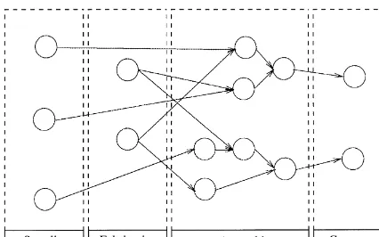
have seen the reduction of "xed cost by down-sizing and outsourcing. Companies now focus on their core competences which are construction, fabrication, and assembly of customer-speci"c in-vestive goods. Fig. 1 shows the supply chain of make-to-order companies with the four levels cus-tomers, assembly, fabrication, and suppliers. On the customer-level there are multiple orders with speci"c due dates. Each order is depicted on the assembly-level by a set of assembly jobs which are interrelated by technological precedence con-straints. To be processed, an assembly job demands scarce assembly capacity as well as in-house fab-ricated and outside procured parts. Holding cost of the assembled parts have to be taken into account. A resource- and precedence-feasible assembly
Fig. 1. Supply-chain of make-to-order companies.
schedule determines the time-phased demand for parts. In-house part fabrication takes place on the third level. Here, multiple parts have to be manu-factured subject to scarce resources while taking into account setup and holding cost. Part ordering from outside suppliers is subject of the fourth level. Relevant cost are ordering and holding cost. The objective is to provide a time- and resource-feasible production plan which respects the due dates while minimizing the cost of the entire supply chain.
The remainder of this paper is as follows. Section 2 provides a more detailed and formal description of the problem. An extensive literature review in Section 3 reveals that the outlined problem has not been treated so far. Hence, Section 4 proposes a mixed integer programming (MIP) formulation of the decision problem and discusses properties of the MIP formulation. Section 5 proposes a two-level, backward oriented, top-down approach in order to solve the problem heuristically. The approach is experimentally evaluated on a set of test instances in Section 6. Finally, Section 7 sum-marizes the results and gives an outlook on further research.
2. Problem description
We will now detail the planning problem in a more formal way by considering each level of the supply chain. In order to keep the amount of nota-tion small, we employ, whenever possible, the same
parameter for the assembly and the fabrication level. Distinction will be made by the superscripts
`Aaand`Fawhich stand for assembly and fabrica-tion, respectively. Table 11 in the Appendix pro-vides a compact overview of the notation. Let us now begin with the customer level.
Customer. From production planning we have
A*0 di!erent customer orders, where order
a"1,2,Ahas the due dated
a*0.
Assembly. Order a is made of assembly jobs
j"s
a,2,ea. The number of all assembly jobs is J"e
A. Due to aggregation, each assembly job jrepresents a set of operations. E.g., in shipbuilding so-called super blocks comprise a number of panel-led or curved blocks (cf. [1]). The assembly of a panelled or curved block is depicted by an opera-tion while the assembly of a super block is depicted by a job. Assembly jobj has a processing time of
p
j*0 and requirescj,r*0 units from theRA*0
di!erent types of assembly resources (assemblers with di!erent skills, power tools) during every time instant it is processed. Job preemption is not al-lowed. Assembly resource typer"1,2,RAhas an
available capacity ofCAr,t*0 units at time instant
t*0. We assume that all events on the customer and the assembly level, i.e., due dates and the change of available capacities, occur at discrete multiples of a standard period length and that the processing times of the assembly jobs are multiples of the standard period length. In this case, the start time of the assembly jobs will be also discrete mul-tiples of the period length.
The assembly jobs are interrelated by an assem-bly network where jobjhas a setP
jof immediate
predecessor jobs. The start of an assembly job at time instant t determines a demand for in-house-fabricated and outside procured parts. The sum of the holdings cost for all parts which are assembled by jobjequals hAj per period. A graphical repres-entation of orders, due dates, and assembly jobs with their technological precedence relations can be given by an integrated assembly graph where each assembly jobjis depicted by a node, and each precedence relation between assembly jobhand its immediate successorj is depicted by an arc hPj
with weightt.*/
h,j"0. We introduce two additional
jobs, a dummy source j"0 and a dummy sink
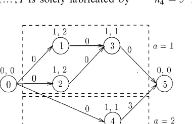
Fig. 2. Integrated assembly graph for an example instance.
each assembly job without predecessors and from
each"nal assembly job to the sinkJ#1. The arcs
from the source have weight 0 while the arcs from
the "nal assemblies e
a(a"1,2,A) to the source
have the weightt.*/
ea,J`1"d.!9!dawhered.!9
de-notes the maximal due date of all orders. With
J"M0,2,J#1Nwe denote the set of all assembly
jobs of the integrated network.
Fig. 2 gives the assembly graph on an example instance with A"2 orders and due dates d
1"5
andd
2"3. The processing timepjand the capacity
requirement c
j,1 w.r.t. the single resource type RA"1 are given above the nodes. The jobs of each order are enclosed by a dotted rectangle, i.e., order
a"1 comprises the assembly jobs 1,2, 3 and
or-dera"2 is made of the"nal assembly job 4. That is, we haves
1"1,e1"3, ands2"e2"4.
Fabrication. An assembly schedule determines a time-phased demand for part types which have to be either manufactured in-house or have to be procured from outside suppliers. The number of part types which are manufactured in-house is
I*0 and the number of part units of type
i"1,2,Ineeded by assembly jobjisqj,i*0. The
in-house fabrication comprisesRFdi!erent produc-tion units. A producproduc-tion unit might be, dependent on the amount of aggregation, an entire job shop or
#ow shop, a set of identical machines such as nu-merically controlled lathes or one physically ma-chine such as a steel burning mama-chine. Production unitr"1,2,RFin periodthas an overall period
capacity ofCFr,t*0 where periodtis the time span between the time instantst!1 andt. The length of a period amounts between one day and one week. Each part type i"1,2,I is solely fabricated by
production unit rFi3M1,2,RFN in a single level
production process. For the production of one unit of part i, a capacity of c
i is needed. Within each
period partiis produced,"xed setup cost ofs iare
incurred. The use of setup time is not explicitly considered because setup times are negligible in the aggregated view. In order to guarantee feasible production plans, we set the available period capa-cityCFr,t not equal the total capacity but we with-draw some capacity in order to obtain slack capacity (cf. [4]). Production of one unit in period
q(tfor a demand in periodtincurs holding cost of
hFi per period.
Supplier. Parts which are procured from outside suppliers have to be available in the period preced-ing the start time of the assembly. The holdpreced-ing cost of all parts which are procured by assembly job
j are hPj per period; for reasons to be explained below,"xed ordering cost do not have to be taken into account.
We extend the example given by the assembly graph of Fig. 2 as follows. There is a single assembly and a single fabrication resource, with a capacity of
CA1,t"3 andCF1,t"10 for each time instanttand period t, respectively. The number of fabricated part types equalsI"3; there are no external pro-cured parts. Production coe$ents, setup and hold-ing cost of the three internal fabricated part types arecF"(1, 1, 1),s"(20, 10, 10), andhF"(1, 2, 1), respectively. The demand for fabricated parts as imposed by the assembly jobs is given in Table 1. According to formula hAj"hPj#+I
i/1hFi )qj,i the
holding cost for the assembly jobs can be calculated tohA1"5)1"5,hA2"5)2"10,hA3"5)1"5, and
Table 1
Part demand of the assembly jobs
i j
1 2 3 4
1 5 0 5 0
2 0 5 0 0
3 0 0 0 5
3. Literature review
There have been di!erent approaches for pro-duction planning of multi-level propro-duction systems. According to the type of the production system regarded at each level, we can discriminate (i) integ-rated project scheduling and part ordering, (ii) multi-level capacitated lotsizing, and (iii) integrated lotsizing and scheduling.
Integrated project scheduling and part ordering. Project scheduling and part ordering depicts the case where on the"rst level multiple projects have to be scheduled subject to precedence and resource constraints. The jobs of the project require parts at the second level. Costs associated with the parts are ordering and holding cost.
Aquilano and Smith [5] were the"rst who integ-rated project scheduling and material requirements planning. Without providing a formal decision model, they depict a single project which has to be scheduled subject to precedence constraints only. The jobs of the project require parts. In order to determine the time-phased demand for these parts, Aquilano and Smith proposed a two-stage ap-proach. First, latest start times for the jobs are calculated by traditional backward recursion (cf. [6]) from the project's due date. The obtained start times determine the gross requirements for parts. The second phase performs calculation of the net requirement by balancing gross requirements, on-hand inventories, and scheduled receipts in a for-ward oriented fashion (cf. [7]). Finally, a lot-for-lot policy is used to calculate planned production quantities for the parts.
Hastings et al. [8] extend this approach. They perform forward oriented scheduling of the jobs by explicitly considering scarce capacities. The
time-phased demand of parts is obtained from the ear-liest precedence and resource feasible start times of the jobs. Hastings et al. coin this approach` sched-ule based materials requirements planningainstead of `lead time materials requirements planninga
which derives the start times of the jobs by un-capacitated backward recursion of jobs from the due date.
Sum and Hill [9] consider multiple projects, scarce capacities on the scheduling level, and lot sizing decisions on the fabrication level. Without providing a decision model, they suggest a two-stage approach. First, backward loading of the jobs subject to capacity constraints is done. Second, three greedy heuristics are proposed in order to perform the order sizing for the time-phased part demand of the jobs.
Smith-Daniels and Smith-Daniels [10] extended the work of Aquilano and Smith [5]. They propose a MIP model for a single project, multi-part order-ing problem where a sorder-ingle project has to be sched-uled such that the sum of holding cost for parts and jobs, ordering cost for parts, and penalty cost for a project delay is minimized. A MIP model is proposed and it is shown that the optimal solution is obtained by realizing a late-start schedule and solving the remainingIsingle-level uncapacitated dynamic lotsizing models to optimality. In an experimental investigation Smith-Daniels and Smith-Daniels compared the optimal solutions to the ones which were obtained by a lot-for-lot strat-egy and showed that the latter resulted in signi" -cantly higher cost.
In [11], the scope of the model is headed towards a cash oriented perspective. The objective function maximizes the net present value of the integrated project scheduling and part ordering model and a new constraint depicts the dynamic cash balance constraint for each period.
observations, Dodin and Elimam device a simple heuristic which, based on the instance at hand, alternatively generates an earliest start or latest start schedule with jobs at normal or at crash duration. The remaining lot-size problems are sol-ved with the part-period heuristic (cf. [13]).
Ronen and Trietsch [14] consider the case where the parts demanded by the jobs can be sourced from di!erent suppliers. Furthermore, the process-ing times of the jobs and the lead time of parts is not deterministic but stochastic. Each part-supplier combination is de"ned by a price and a lead time distribution. Holding cost accrue if parts arrive ahead of the time needed by the job. If late parts delay the project beyond its due date, lateness cost are debited. The decision problem is, to choose for each part a supplier and an ordering time such that the total expected cost are minimized. Assuming that the variability of the processing times is negli-gible, Ronen and Trietsch propose the following solution procedure. First, latest start times of the jobs are computed by backward recursion from the project's due date (cf. [6]). Then, order times for each part are computed, and "nally, a supplier is chosen for each part. The method is embedded in a decision support system (cf. [14]).
Multi-level capacitated lotsizing. Multi-level capacitated lotsizing models depict a production system with multiple levels where on each level lotsizing rather than scheduling decision have to be undertaken. Given are the demands for multiple parts (which are usually referred to as items) where each part is depicted by a multi-level product struc-ture. Each part within the product structure has to be fabricated on one level of the production system. Since there is no a priori lot size, any amount of a part can be produced as long as the capacity constraints are respected. Production of a part in-curs setup cost and in some cases setup times; part inventories incur holding cost. The problem is to obtain a cost minimal production plan which re-spects the scarce capacities of the resources on all levels of the production system and delivers "nal demand parts without backlogging. Models and methods for this intricated problems can be distin-guished w.r.t. the type of product structure allowed and w.r.t. the amount of aggregation. Regarding the product structure, general product structures
and assembly product structures can be distin-guished. Regarding the amount of aggregation, so-called big bucket and small bucket models can be distinguished (cf. [15]). Big bucket models such as the capacitated lotsizing problem (CLSP) have a rather high aggregation level where one period amounts about a week. Here, scheduling decision which determine the sequence of production lots in one period are not taken into account. Contrary, in small bucket models a period embraces a smaller time span and the planning problem is to simulta-neously determine lot sizes and lot sequences in each period. Multi-level big bucket problems with general product structures have been addressed in [4,16}21]. Helber [20], and ZaKpfel [22] give a cash-#ow oriented model where the net present value is maximized. Work on special big bucket prob-lems where either serial or assembly product struc-tures are taken into account or constrained resources are only considered on one production level can be found, amongst others, in [23}27]. Work on multi-level, small bucket models with general product structures has been presented by Kimms [28].
Integrated lotsizing and scheduling. Lasserre [29] introduces a model which integrates the lotsizing decision on an aggregated decision level and the scheduling decision on a detailed decision level. The lotsizing decision is modelled as a multi-part, single level CLSP and the scheduling decision is modelled as a job shop problem (JSP) (cf., e.g., [30]). The production decisions for one period in the lotsizing model determine an entire JSP. Dauze`re-PeHres and Lasserre [31] propose a solu-tion method which alternates between solving the lotsizing problem for a"xed sequence of the jobs at the machines and solving the scheduling problem for given lotsizes.
From the literature review we can see that the problem of a heterogenous production system where multiple customer speci"c projects have to be scheduled subject to scarce capacities on the"rst level and where capacitated lotsizing of multiple parts has to be done on the second level such that the cost of the entire supply chain are minimized has not been treated so far. In what follows, we will
"rst propose an MIP formulation of the problem
4. An integrated model
4.1. MIP formulation
To model the integrated assembly and fabrica-tion problem, we introduce the following decision variables. First, for the assembly we have the binary decision variable x
j,t which equals 1, if job j is
started at time instantt, and 0 otherwise (cf. [32]). We can reduce the number of decision variables by calculating for each jobjan earliest start timeES
j
and a latest start time¸S
j by traditional forward
and backward recursion (cf. [6]) fromt"0 and the maximal due dated.!9, respectively. Second, for the fabrication we use the production variableQ
i,t*0
which gives the quantity of part typeiproduced in periodt, the inventory variableI
i,t*0 which gives
the quantity of part typeiwhich is in inventory at the end of periodt, and the binary set up variable
y
i,twhich is 1, if production for part typeiin period ttakes place, and 0 otherwise. We can now model the integrated assembly and lotsizing problem (IALP) as follows:
Eqs. (1)}(10) model a two-level supply chain with heterogenous production segments. The model comprises four main parts: (i) the project scheduling based assembly on the"rst level, (ii) coordination of fabrication and assembly, (iii) the lotsizing based fabrication on the second level, and (iv) the objec-tive function which minimizes the sum of holding and setup cost of the entire supply chain. Let us analyze these parts in more detail.
Ad (i). The project scheduling based assembly is depicted by the constraints (2)}(5) and (9). Con-straint (2) assures that each order is "nished not later than its due date. (3) secures that the "nal assembly cannot be delivered to the customer be-fore each assembly job has been executed exactly once. The integrated assembly graph is given by constraint (4). (5) models the capacity constraint of the assembly resources. Finally, constraint (9)
de"nes the binary decision variables.
Ad (ii). Eq. (6) links the part #ow between the fabrication and the assembly. The start of assembly job j at time instant t imposes demand for fab-ricated parts at the end of periodtwhich has to be
ful"lled from the inventory available at the end of
periodt!1 or from fabrication in period t. Ad (iii). Constraints (7), (8) and (10) depict the fabrication. The capacity constraints are given in (7). Constraint (8) sets the binary setup variable
y
i,t"1 when production for part typeitakes place
Fig. 3. Holding cost within the supply chain.
Fig. 4. Optimal solution for the IALP.
Ad (iv). The cost function (1) mimizes the overall production cost which are made of holding cost within the assembly as well as holding and setup cost within the fabrication. Fig. 3 details the accounting of the cost. The due date of the order is 9. Assembly jobjis started at time instantt"5 and the required part typeiis fabricated in periodt"3. Additionally, assembly job j requires a procured part which has to be available at the end of period 5. Within the fabrication, parti is available at the end of periods 3 and 4. Within the assembly, part
iand the procured part are available at the end of periods 5,2, 9. Setup cost occur in period 3 where
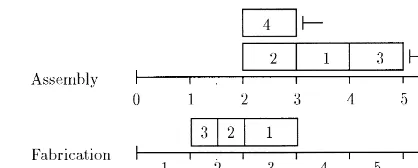
partiis produced. Ordering cost for the procured part are not taken into account. If order cost are relevant for a procured part, we depict this part as an additional in-house fabricated part with a capa-city demand of 0 on a dummy fabrication resource. Solving the example instance introduced above with IALP to optimality, we obtain the solution given in Fig. 4 with overall cost of 120 which are made of 40 units setup cost, 5 units fabrication holding cost, and 75 units assembly holding cost.
4.2. Model properties
In this section we will look at some properties of the integrated assembly and lotsizing problem. Let us begin with two subproblems of the IALP which are well knownNP-hard optimization problems. Consider"rst the assembly scheduling problem (ASP) on the"rst level. The ASP is depicted by the
"rst term of the objective function (1) as well as
constraints (2)}(5) and (9). The ASP models the assembly with the objective to minimize the
assem-bly wide holding cost. It is the`mirror problemaof the well known resource-constrained project sched-uling problem (RCPSP) where the latter has the objective of minimizing the sum of the weighted job
#ow times (cf. [33,34]). The RCPSP can be poly-nomially obtained from the ASP by giving each job
jthe new job numberJ#1!j, reversing all arcs
hPjtojPh, and keeping everything else as it is. It is well known that the RCPSP is an NP-hard optimization problem (cf. [35]). A survey of exact and heuristic solution procedures for the RCPSP with di!erent objective function values can be found in Kolisch and Padman [36].
Consider now, the fabrication lotsizing problem (FLP) on the second level. The FLP is depicted by the second term of the objective function (1) as well as constraints (6)}(8) and (10) where we assume that the x
j,t values in the coupling constraints (6) are
parameters. The FLP models theRFdi!erent pro-duction units of the fabrication with the objective to minimize the fabrication wide holding and setup cost. Since each parti is manufactured on exactly one of the production units, namely rFi, we have
RFseperate optimization problems. Each of it is the well known single-level multi-part capacitated lot-sizing problem (CLSP) (cf. [37]) which is strongly
NP-hard (cf. [38]). Optimal methods proposed to solve the CLSP are, amongst others, valid inequali-ties (cf. [39]), network #ow formulation (cf. [15]), branch-and-bound (cf. [40]), cross decomposition (cf. [41]), as well as linear programming, column generation, and subgradient optimization (cf. [38]). A survey of heuristic approaches for the CLSP will be given in Section 5.2.
Fig. 5. Optimal sequencial solution.
Moreover, the presence of due dates makes the feasibility problem of the IALP alreadyNP -com-plete.
De5nition 1. Right-regular. An objective function
Zis right-regular i! the following holds. For each pair of two feasible schedules S"(S
1,2,SJ) and S@"(S@
1,2,S@J) with Sj)S@j for a single job j
and S
i"S@i for the remaining jobs i"1,2, j!1,j#1,2,Jthere isZ(S))Z(S@).
Theorem 1. The objective function(1)is right-regu-lar.
Proof. Consider a feasible assembly schedule
Swhere jobjhas the start timeS
j. Changing, c.p.,
the start time toS
j#1 will decrease the"rst term
of the objective function byhAj. For the second term we can reason as follows. The fact that, c.p., the part demand of job j occurs at time instantS
j#1
in-stead ofS
jenlarges the solution space (2), (3)}(5) of
the FLP. Hence, for the new assembly schedule, the second term of the objective function must be less equal than the one of the former assembly schedule. h
Theorem 2. The optimal sequential solution of the ASP and the FLP, i.e.,xrst solving ASP and thereafter FLP to optimality, does not guarantee an optimal solution of the integrated assembly and lotsizing problem.
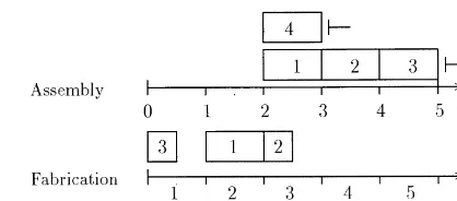
Proof. We prove Theorem 2 by showing that the optimal sequential solution of the example instance given in Section 2 is not an optimal solution for the IALP. We "rst solve the ASP to optimality and obtain an assembly schedule with holding cost of 70. This is 5 units better than the assembly schedule of the optimal IALP solution (cf. Section 4.1). The subsequent optimal solution of the remaining FLP gives rise to a production plan with setup cost of 40 and holding cost of 15 and hence overall fabrica-tion cost of 55. Fig. 5 illustrates the solufabrica-tion with a Gantt-chart. The total cost for the entire supply
chain are 125 which are 5 units more than the optimal solution of the IALP. Note that the sequen-tial solution has the same setup cost as the optimal IALP solution and hence looses its optimality by higher holding cost solely. h
Theorem 3. Solving the assembly scheduling problem to optimality might produce an infeasible fabrication lotsizing problem.
Proof. Again, we use a counterexample in order to prove Theorem 3. We consider a single orderA"1 with d
1"4, J"3, RA"1,RF"1,CA1,t"1 for
each time instantt*0 andCF1,t"10 for each peri-od t"1,2, 4. The precedence relations between
the jobs are the same as for order a"1 of the assembly graph given in Fig. 2. Furthermore, we have I"2 parts with production coe$cients
C
1"C2"1 on the single fabrication resource,
part demands of q
1"(5, 0),q2"(0, 15), and q
3"(10, 0), a processing time ofpj"1 for each job j, part setup cost ofs"(10, 10), and part holding cost ofhF"(4, 1). Solving the ASP to optimality, we obtain the assembly schedule on the left side of Fig. 6. For this schedule there does not exist a feas-ible FLP-solution since assembly job 2 requires 15 units of part type 2 at the end of period 1 and the fabrication capacity in period 1 is onlyCF1,1"10. The right side of Fig. 6 gives an optimal and feasible IALP-solution for the problem. h
5. Solution methodology
Fig. 6. Infeasible sequential and optimal integrated solution.
the IALP into its two subproblems, the ASP and the FLP. A two-level approach"rst determines an assembly schedule and afterwards lotsizes for the FLP. The coordination of the levels is in a strict top-down fashion with no feedback from the subor-dinate level (cf. [42]). Also, there is no explicit feasibility anticipation on the "rst level, but only a cost anticipation. Both levels perform a backward oriented planning approach.
5.1. A list scheduling heuristic for the assembly scheduling problem
We use a backward oriented list scheduling heu-ristic (cf. [43]) which schedules the jobs sequentially in the order given by a job list p at their latest precedence and resource feasible start times. Two issues need clari"cation. First, how to construct a list, and second, how to transform a list into a feasible schedule. Let us begin with the construc-tion of a feasible list.
5.1.1. List generation
A list n"Sj
1,j2,2,jJ] consists of the J
non-dummy jobs wherej
gis the job at list positiong. In
order to transform a listninto a feasible schedule
S"(S
1,2,SJ), the list has to respect the
technolo-gical precedence constraints as imposed by the as-sembly graph. Let for job j be S
j the set of
immediate successor jobs. Then
S
jg-Mj1,2,jg~1N (g"2,2,J) (11)
states that job j must have a greater list position than each of its direct successor jobs. By transitiv-ity, the list position of jobjis also greater than each of its indirect successor jobs. Let L(0)"MJ#1N
and let L(g)"MJ#1,j
1,2,jgN denote a set of
jobs comprising the dummy sink of the integrated assembly network and all jobs which have been put to list positions 1,2,g. Let further beA(g) the set
of all available jobs which can be put at list position
g. On account of Eq. (11)A(g) can be de"ned as
A(g)"Mj3JDjNL(g!1) andS
j-L(g!1)N.
(12) That is, available jobs itself must not be on the list, while all their successor jobs have to be on the list. Denoting withv(j) a priority value associated with jobj we can give the list generation algorithm as follows:
List Generation
A.Initialization:L(0)"MJ#1N. B.Iteration: For g"1 toJ do
(1) UpdateA(g). (2) Selectj
g3A(g) withv(jg)"maxi|A
(g)v(i).
(3) UpdateL(g).
The Initialization de"nes the setL(0) to include the dummy sink of the integrated assembly network only. Step (1) updates the set of available jobs, Step (2) selects one job from the available set and puts it in list positionj
g. In case of ties, Step (2) selects the
job on the basis of`"rst come"rst servea(FCFS) where the job is preferred which has been"rst in the set A(g). Further ties are resolved by picking the job with the smaller job number. Step (3) updates the set of jobs on the list.
Table 2
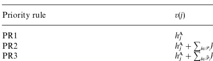
Priority rules for list generation
Priority rule v(j)
PR1 hAj
PR2 hAj#+i|PjhAi
PR3 hAj#+
i|PIjhAi
Table 3
List generation for the example instance
g 1 2 3 4
L(g!1) M5N M3, 5N M2, 3, 5N M2, 3, 4, 5N
A(g) M3, 4N M1, 2, 4N M1, 4N M1N
j
g 3 2 4 1
jobs.PI
jdenotes the set of all predecessors of jobj.
Using priority rule PR3 for the four non-dummy jobs of the example instance, we obtain the priority values v(1)"5, v(2)"10, v(3)"20, and v(4)"5. Table 3 details the list generation of the example instance when these priority values are employed. The resulting list isn"S3, 2, 4, 1].
5.1.2. Schedule generation
We now want to transform listninto a feasible schedule S(n) which gives a start timeS
j for each
jobj such that precedence relations, the assembly resource constraints, and the order due dates are taken into account. Given the listp, we can simply schedule the jobs in the order of the list at their latest feasible start times. To do so, we need to knowCIAr,t(g), the available capacity of the assembly resourcerat time instanttwhen scheduling thegth job from the list. For the job on list positiong"1 the available capacityCIAr,t(1) is equal to the initial capacity CAr,t for all resource types r and time in-stants t. For the jobs on list position g"2,2,J
the available capacity is dynamically updated ac-cording to
CIAr,t(g)"CIAr,t(g!1)
!
G
c
jg~1,r ift3MSjg~1,2,Sjg~1#pjg~1!1N,
0 else,
r"1,2,RA, t"0,2,¹. (13)
The schedule generation algorithm can be given as follows.
Schedule generation(p) A. Initialization: S
J`1"maxAa/1da,¹"SJ`1!1, CIAr,t(1)"CAr,tforr"1,2,RA,t"0,2,¹.
B.Iteration: For g"1 toJ do (1) CalculateCIA
r,t(g) according to (13).
(2) Take the next job from the list:j"j g.
(3) Determine the dynamic latest start time¸S@ jof
jw.r.t. precedence constraints:
¸S@ j"min
k|S j
MSk!t.*/ j,kN!pj.
(4) Determine the latest resource feasible start time
S
jofjwhich is)¸S@j: S
j(¸S@j)
"maxLS@
j
t/ESjMtDr"1,2,RA;
q"t,2,t#pj!1:CIAr,q(g)*cj,rN.
The Initialization sets the start time of the sink to the maximal due date, sets the planning horizon to the time instant before the start time of the sink, and sets the available capacity equal the initial capacity. Afterwards, Steps (1)}(4) are performed
Jtimes. At iterationg, jobj
gis scheduled as late as
possible. Step (1) updates the available capacity. Step (2) takes the next jobjfrom the list. Step (3) determines the dynamic latest start time ¸S@
j
ac-cording to precedence relations and due dates as depicted in the assembly graph. Finally, Step (4) searches for the latest start time of jobjwithin the time window [ES
j,¸S@j] where ESj is the static
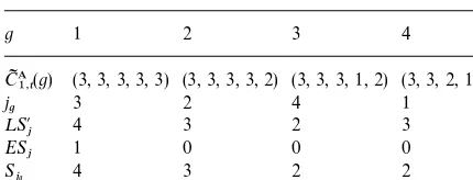
earliest start time of jobjas calculated by forward recursion (cf. [6]). Table 4 details the scheduling algorithm when applied with listn"S3, 2, 1, 4] to the example instance. The second row gives the available capacity CIA1,t(g) of the single resource
r"1 for time periods t"1,2, 5. The assembly
schedule which is generated isS"(2, 3, 4, 2). It has assembly wide holding cost of 70 and is given in the upper part of Fig. 5.
Table 4
Schedule generation for the example instance
g 1 2 3 4
CIA1,t(g) (3, 3, 3, 3, 3) (3, 3, 3, 3, 2) (3, 3, 3, 1, 2) (3, 3, 2, 1, 2)
j
g 3 2 4 1
¸S@j 4 3 2 3
ES
j 1 0 0 0
S
jg 4 3 2 2
De5nition 2. Right-active schedule. A right-active schedule is a feasible schedule where none of the jobs can be started later without forcing at least one other job to start earlier.
Theorem 4. The schedule generation algorithm gen-erates schedules which are right-active.
Proof. The schedule generation algorithm gener-ates right-active schedules by construction because each jobjis scheduled as late as possible.
Since the objective function (1) of the IALP is right-regular, there exists one listnHwhich is map-ped by the schedule generation algorithm into the IALP-optimal assembly schedule. Note, that a given listpmight lead to an infeasible solution of the ASP or IALP.
5.2. A backward oriented heuristic for the fabrication lotsizing problem
Given an assembly scheduleS, the time-phased part demand is
D i,t"
J + j/1@Sj/t
q
j,i (14)
and what remains is to solve RF independent CLSPs. There have been many heuristics suggested to solve the CLSP. A survey can be found in [45,46]. Roughly, we can divide heuristic ap-proaches in construction heuristics, improvement heuristics, and mathematical programming based heuristics. Construction heuristics build a feasible
production plan by proceeding from period to peri-od and deciding via cost values about the lot sizes of parts in the current period. Examples of such approaches are given in [47}51]. Contrary to the period-by-period approach, the heuristic of Kirca and KoKkten [52] performs a part-by-part approach where it is proceeded from one part to the next and for each part a production plan for the whole planning horizon is constructed.
Improvement heuristics start with a not neces-sarily feasible production plan and try to alter it
"rst to a feasible production plan and afterwards to
a production plan with less total cost by shifting production lots. Examples of improvement heuris-tics are given in [53,54].
Finally, mathematical programming based heu-ristics construct for each part a number of produc-tion plans. The capacity feasible and cost minimal coordination of production plans is obtained by employing each production plan as column in a large-scale linear program. Examples are given in [46,55]. A special case are approaches where,"rst, optimal setup patterns are found for the un-capacitated lotsizing problem and afterwards production quantities are found by solving a trans-portation problem (cf. [56]).
Here, we will suggest a two-phase, backward oriented, period-by-period heuristic. The"rst phase constructs a feasible production plan and the sec-ond phase tries to improve this plan by greedily shifting production lots. Both phases work in a backward oriented manner. The idea of backward oriented construction heuristics to solve capacitated lotsizing problems has been "rst given by Haase [57] and later extended by Kimms [28]. Its advant-ages are twofold. First, for the IALP, backward planning is more intuitive than forward planning. Second, contrary to forward oriented methods, we do not have to employ time consuming feasibility routines.
5.2.1. Lotsizing generation scheme
As pointed out above, the lotsizing heuristic comprises a construction and an improvement phase. The basic idea of the construction phase is to step backward from the latest demand period¹to period 1. In each period t"¹,2, 1 we decide
produced now and for which parts we should shift the demand into the next prior demand period. We make this decision based on a cost value. The second phase is similar but has two exceptions. First, instead of demands, it tries to shift produc-tion lots and, second, shifting is not restricted to the next prior production period but to all prior pro-duction periods. In order to give a formal descrip-tion of the algorithm let us use some notadescrip-tion. We begin with the calculation of the time-phased demand as given in Eq. (14). The time-phased de-mand unfolds a cumulated capacity dede-mand of
CD
r,t w.r.t. fabrication resource r between period
1 and periodt
The cumulated capacityCCF
r,tof resourcerbetween
period 1 and tis
t with positive demand in t is I
t"Mi3IDDi,t'0N. Being in periodtand looking
&backward'in time, we determine for parti3I
tthe
next periodq
i(twith positive demand q
i"(M0NXmaxMqDq"1,2,t!1:Di,q'0N). (17)
If there is no more part demand in periods 1,2,t!1, thenqiis set to 0. Let denoteBtthe set
of demands in periodtwhich can be shifted back-wards, i.e.,
wheredi is a part speci"c cost saving value whose calculation will be detailed in Section 5.2.2. We can now outline the backward lotsizing algorithm in a more formal way. Note that for a given assembly schedule S, we will use the time-phased demand array D
i,t in a dynamic fashion. That is, the lot
sizing heuristic will alterD
i,tby moving and
delet-ing demands. Whenever a change in the demand matrix takes place, I
t, CDr,t, and Bt as de"ned
above are updated.
Backward lotsizing(r)
A. Initialization: Set ¹ equal the latest demand period.
B.Construction phase: Fort"¹to 1 do (1) WhileB
t"~do
Select onei3B
tbased on the cost
saving valued
Determine the amount ofi producable in t:Q
After the initialization has been completed, steps (1)}(2) are performed ¹times. In each iterationt, Step (1) iteratively selects the part typei from the set of backshiftable demands which maximizes the cost measure d
i and shifts the associated demand D
i,tto the prior demand periodqi. When there are
no shiftable demands left, Step (2) determines pro-duction lots for the remaining parts with demand in periodt. The selection criterion is the holding cost per used capacity unith
i/ci. If a demandDi,tcannot
be entirely produced intbut has to be splitted, it is checked whether a cost saving can be achieved by shifting the entire demandD
i,tto the prior period
t!1.
The improvement phase builds up on the pro-duction plan obtained after the¹-th iteration has been performed. It systematically checks for each partiwith positive lot size in periodt"¹,2, 2, if
the total fabrication cost can be reduced by shifting the production lot Q
i,t to a production period q"t!1,2, 1. Each improvement of the
Table 5
Backward lotsizing for the example instance
t I
t Step
(1) (2)
i qi di B
t Di,t Di,qi i Qi,t Di,t Di,t~1
t"4 M1N 1 2 2 M1N 0 10
t"3 M2N MN 2 5 0 0
t"2 M1, 3N MN 1 10 0 0
3 0 5 0
t"1 M3N MN 3 5 0
Table 5 shows the functioning of the backward lotsizing heuristic when applied to the example instance with the demands D
1"(0, 5, 0, 5,), D
2"(0, 0, 5, 0),D3"(0, 5, 0, 0) and when
employ-ing the Dixon}Silver cost criterion (cf. Section 5.2.2). The demands stem from the heuristically derived assembly schedule of Section 5.1.2. Note that after the construction phase there is no im-provement phase because each part is produced in a single period. The lotsizing policy obtained has overall cost of 55 which gives total cost for the IALP of 125. The production plan, comprising assembly schedule and fabrication lotsizes, is the same as derived by solving the IALP sequentially. Fig. 5 visualizes the solution.
5.2.2. Cost considerations
In order to decide if partishall be produced in the current periodtor shall be backshifted to the next prior demand period q
i, we have employed
di!erent cost valuesd
i. Namely, these are adapted
cost calculations of the period-by-period ap-proaches of Eisenhut [47], Dixon and Silver [49], GuKnther [50] as well as Lambrecht and Vander-veken [48]. Originally, all of them take setup and holding cost in a forward oriented period-by-peri-od approach into account. Here, we will adapt them to our backward oriented approach. For each partiwe will only compare two alternatives: pro-duction of the demand D
i,t in the current period tand backshifting of the demandD
i,tto the prior
demand periodq
i(t. Note that the demand vector D
i for part i might be sparse and hence qi and tmight not be adjacent periods, i.e.,t!q
i'1.
The cost measure of Dixon and Silver [49] employs the Silver}Meal criterion [58] for the uncapacitated LSP which compares the average cost per period when producing the demandD
i,tin tor inq
i. Production intincurs per period cost ofsi,
production in q
i incurs per period cost of
(s
i#hi)Di,t)(t!qi))/(t!qi#1). The per period
cost saving when producing in q
i instead of t is s
i!(si#hi)Di,t)(t!qi))/(t!qi#1). Dixon and
Silver generalize this measure for the capacitated case by dividing it by the number of capacity units employed to produce the demandD
i,t:
dDSi "
s i!
s
i#hi)Di,t)(t!qi)
t!q
i#1 c
i)Di,t
. (19)
Eisenhut [47] employs the total cost saving when producing the demandD
i,t in qi instead oft. The
total cost saving equals s
i!hi)Di,t)(t!qi). This
value is divided by (t!q
i#1)2)ci)Di,tin order to
derive the following cost measure:
dEi"si!hi)Di,t)(t!qi)
(t!q
i#1)2)ci)Di,t
. (20)
Lambrecht and Vanderveken [48] extend the cost measure of Eisenhut as follows:
dLVi " si!hi)Di,t)(t!qi)2
c
i)Di,t)(t!qi#1))(t!qi)
. (21)
Table 6
DF-setting for small large instances
RSA" Small Large
0.1 0.3 0.5 0.1 0.3 0.5
RSF"0.1 0.50 0.45 0.40 0.40 0.35 0.30
RSF"0.3 0.45 0.40 0.35 0.35 0.30 0.25
RSF"0.5 0.40 0.35 0.30 0.30 0.25 0.20
marginal decrease of the per period setup cost equals the marginal increase of the per period hold-ing cost. Gro! transfers this idea to the dynamic uncapacitated LSP and GuKnther [50] extends this approach to the capacitated lotsizing problem. Adapting the idea of GuKnther to the backward oriented approach, we derive the following cost measure:
Additionally, we have altered cost measure (22) slightly to depict the cost saving (CS) per covered period divided by the capacity demand.
dCSi "
To illustrate the calculation of the di!erent cost measures let us look at iterationt"4 of the back-ward lotsizing heuristic as given in Table 5. Here, we havei"1,h
i"1,si"20,t"4,qi"2,Di,4"5,
andc
i"1. According to the formulas given above,
we obtain the cost measures dDS1 "2,dE1"2/9,
dLV1 "0,dG1"5, anddCS1"1/3.
6. Experimental evaluation
6.1. Test Instances
For evaluation purposes, a set of 270 problem instances was generated with a parameter control-led instance generator for assembly type problems which builds up on ProGen (cf. [61]). The instance set can be divided w.r.t. the size into small and large instances. A full factorial experimental design with three independent problem parameters was em-ployed for both sets. The three independent prob-lem parameters are the constrainedness of the assembly resources, the constrainedness of the fab-rication resources, and the ratio of setup and hold-ing cost. All other parameters were randomly drawn from given intervals.
For the small test instances, there is A"3,
J
a3[3, 5],I"4,RA"1,RFA"1,RF"1,PF"0.5,
andr
a3[0, 10].Jadenotes the count of jobs
belong-ing to each order, RFA denotes the assembly resource factor for all jobs. RFA measures the density of the capacity demand arrayc
j,rfor
assem-bly resources (cf. [61]). Correspondingly, PF
denotes the part factor which measures the density of the part demand array q
j,i.RFA"1 expresses
the fact that all non-dummy jobs require each of the available resource types in order to be pro-cessed. PF"0.5 says that each non-dummy job requires a positive amount of half of the available part types.
The following parameters were randomly drawn from the speci"ed intervals: p
j3[1, 3],cj,r3[1, 3], q
j,i3[10, 50]. The due date da was calculated as
follows. First, an order speci"c release date r awas
randomly drawn from the uniformly distributed interval [0, 10]. Afterwards,dM, an upper bound of the completion of all orders if started at time in-stantt"0 is computed by summing up the pro-cessing times of of jobs, i.e.,dM"+J
j/1pj. Now, da,
the due date of order a, is computed to
d
a"ra#¸Psa,ea#DF(dM!¸Psa,ea) where¸Psa,ea
de-notes the longest path from the start jobs ato the
end job e
aof order aand DF3[0, 1] denotes the
due date factor. To generate feasible instances,DF
has been set according to the scarcity of assembly and fabrication resources as given in Table 6.
The large problem instances are characterized by the following parameter values:A"10,J
a3[5, 10], RA"2,RF"2,I"8, andr
a3[0,30]. The due date
factorDFhas been set according to Table 6. The three independent problem parameters are
The assembly resource strength RSA measures the scarcity of the assembly resource capacity given in constraint type (3). ForRSA"0, the capacity for each resource typerequals the minimum capacity needed when no two jobs are processed in parallel. For RSA"1, the capacity for each resource type
rsu$ces to realize the scheduleS"(¸S
1,2,¸SJ)
where each job j starts at the latest precedence feasible time instant ¸S
j in order to "nish each
orderaat its due dated
a.RSAhas been set to 0.20,
0.35, and 0.50.
The fabrication resource strengthRSFmeasures the available capacity of the fabrication resources given in constraint type (8). ForRSF"1, the capa-city of the fabrication resources is su$cient in order to realize a cost-optimal Wagner}Whitin schedule for the time-phased part demand as induced by the schedule S"(¸S
1,2,¸SJ). For RSF"0, there
is just enough capacity in order to produce the demand as given by assembly schedule S"
(¸S
1,2,¸SJ). RSFhas been set to 0.20, 0.35, and
0.50.
Finally,TBO, the time between order, determines the ratio of holding and setup cost according to the following formula (cf. [20,62,63]):
s
i" 0.5)hi +Jj
/1qj,i
¹ )¹BO2 . (24)
TheTBOhas been set to 1, 3, and 5.
Realizing a full factorial design with 5 replica-tions for each combination of the independent parameter levels, 5)33"135 instances were gener-ated for the small and the large instance set, respec-tively; in total we employed 270 instances. Each instance was solved with each combination of the 3 priority rules and the 5 cost measures. In the sequel we will refer to a`scheduling heuristicawhen employing the list scheduling heuristic with one priority rule and to a `lotsizing heuristica when employing the backward lotsizing algorithm with one particular cost measure. As a `heuristica we coin each combination of a scheduling and a lotsiz-ing heuristic. Additional to these heuristics, we tested the combination of each scheduling heuristic with the lotsizing algorithm of Kirca and KoKkten [52]. The latter method showed very favourable results when compared to the heuristics of
Lam-brecht and Vanderveken [48], Dixon and Silver [49], Maes and Van Wassenhove [51], and Cat-trysse et al. [55]. In total we run 270)3)6"4860 experiments. Due to the fact that the feasibility problem of the IALP is NP-complete, we could solve only 116 of the small and 130 of the large instances by each of the 3)6"18 tested heuristics to feasibility. To obtain lower bounds, we solved for each small instance the model (1)}(10) with the relaxation 0)y
i,t)1 with CPLEX (cf. [64]).
Upper bounds were obtained by selecting for each instance the best objective function value obtained by one of the 18 heuristics and a tabu search procedure (cf. [65]).
If not stated di!erently, we provide means; stat-istical testing was done with nonparametrical tests solely because inspection of the distribution func-tions revealed that none of the values was normally distributed (cf. [66]). In particular, we employed the following tests (cf. [67]). The Wilcoxon matched-pairs signed-ranked test for 2 related samples, the Friedmann test fork'2 related samples, and the Kruskal}Wallis-H test with tie correction fork'2 independent samples. If no level of con"dence is given explicitly, the 1% level of con"dence is meant. All testing was done with SPSS [68].
6.2. Results
We divide the analysis in an assessment of the performance of the 18 di!erent heuristics (Section 6.2.1) and the investigation of the in#uence of the independent problem parameters on the best heuristic proposed in this study (Section 6.2.2).
6.2.1. Performance of the heuristics
Tables 7 and 8 provide three di!erent types of information. First, they give the average deviation of the 18 tested heuristics from the lower and upper bound, respectively. Second, they provide under
avgthe average of all 6 lotsizing heuristics for one scheduling heuristic and of all 3 scheduling heuris-tics for one lotsizing heuristic, respectively. Third,
Table 7
Average deviation from the lower bound-small instances
DS E CS G KK LV avg sig
PR1 26.68 22.18 21.29 22.96 20.82 21.50 22.57 0.00 PR2 26.68 21.89 20.99 22.57 20.28 21.25 22.28 0.00 PR3 26.90 22.24 21.42 22.90 20.83 21.68 22.66 0.00
avg 26.75 22.11 21.23 22.81 20.64 21.47
sig 43.79 57.16 43.25 22.82 24.06 63.32
Table 8
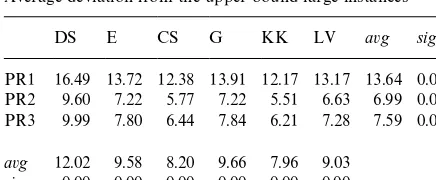
Average deviation from the upper bound-large instances
DS E CS G KK LV avg sig
PR1 16.49 13.72 12.38 13.91 12.17 13.17 13.64 0.00 PR2 9.60 7.22 5.77 7.22 5.51 6.63 6.99 0.00 PR3 9.99 7.80 6.44 7.84 6.21 7.28 7.59 0.00
avg 12.02 9.58 8.20 9.66 7.96 9.03
sig 0.00 0.00 0.00 0.00 0.00 0.00
Table 7 presents the deviation from the lower bound for the small instances. The scheduling heu-ristic PR2 slightly gives the best results; for none of the lotsizing heuristic the use of the scheduling heuristic shows a signi"cant in#uence. Contrary, the use of the lotsizing heuristic has a signi"cant impact on the solution quality. The lotsizing heu-ristic of Kirca and KoKkten (KK) provides the best results followed by the new heuristic (CS). The best 5 integrated scheduling and lotsizing heuristics are PR2/KK (20.28%), PR1/KK (20.82%), PR3/KK (20.83%), PR2/CS (20.99%), and PR2/LV (21.25%).
Table 8 shows the average deviation from the upper bound for the large instances. The scheduling heuristic PR2 gives again the best results; schedul-ing heuristics PR2 and PR3 show signi"cantly bet-ter results than PR1 (sig"0.00) for all lotsizing heuristics. No signi"cant di!erence for PR2 and PR3 was observed for any lotsizing heuristic. Again, the use of the lotsizing heuristic has a signi" -cant impact on the quality of the solution. The best results were obtained with the heuristic of Kirca
and KoKkten (KK) closely followed by the new heu-ristic (CS). The best 5 integrated scheduling and lotsizing heuristics are PR2/KK (5.51%), PR2/CS (5.77%), PR3/KK (6.21%), PR3/CS (6.44%), PR2/LV (6.63%), and PR2/E as well as PR2(G) (7.22%).
6.2.2. Ewect of the problem parametersss
In order to show the e!ect of the independent problem parameters on the heuristics, we have selected PR2/CS as the best performing heuristic of our two-level, backward oriented scheduling and lotsizing approach. Table 9 gives the average devi-ation from the lower bound for the di!erent levels of the three problem parameters. The following observations can be made w.r.t. the in#uence of the three independent problem parameters.
The assembly resource strengthRSAhas only for low TBO- and RSF-levels, i.e., TBO"1 and
RSF"0.20, a systematic but no signi"cant (sig"32.63) in#uence on the performance where a decrease in theRSA-level enforces an increase in the percentage deviation. In other words, if the fabrication is highly resource-constrained and setup cost are negligible, then scarcer assembly capacity will lead to poorer heuristic solutions. This is intuitive, since poor assembly scheduling decisions will raise holding cost in the assembly. Scarce fabrication resources without noteworthy setup cost will transmit and intensify this e!ect.
The fabrication resource strength RSF shows only for highTBO- andRSA-levels, i.e.TBO"3 and
RSA"0.50, a systematic but no signi"cant (sig"69.07) in#uence on the performance where an increase in theRSF-level enforces an increase in the percentage deviation. In other words, if there is abundant fabrication capacity and setup cost are high, the lotsizing heuristics can make many plann-ing mistakes which lead to poor solutions. The e!ect is blurred in the case of scarce fabrication resources or low setup cost.
The time between order TBO is the only para-meter which shows for all combinations of the other two parameter levels a highly signi"cant ef-fect on the heuristic performance. Increasing setup cost leads to a decrease in the solution quality.
Table 9
E!ect of the problem parameters on PR2/CS
TBO"1 TBO"2 TBO"3
RSF RSF RSF
0.20 0.35 0.50 0.20 0.35 0.50 0.20 0.35 0.50
RSA"0.20 7.48 6.41 6.74 20.43 18.74 13.78 29.07 36.75 36.44
0.35 3.56 3.20 4.75 18.78 17.14 21.24 39.39 45.07 32.15
0.50 3.00 3.37 5.83 15.21 18.22 16.66 34.67 36.01 40.10
Table 10
E!ect of the problem parameters on assembly wide holding cost
RSA RSF TBO avg
0.20 0.35 0.50 0.20 0.35 0.50 1 3 5
PR1 5.47 3.57 2.11 4.75 2.89 3.33 3.13 4.53 3.31 3.68
PR2 4.52 2.95 1.76 2.67 3.36 3.10 2.78 2.84 3.44 3.05
PR3 6.06 2.43 1.69 2.80 3.98 3.28 3.87 3.02 3.25 3.36
we solved the"rst term of the objective function (1) as well as constraints (2)}(5) and (9) and calculated the average deviation from the optimum. The latter was obtained by solving the same model with CPLEX.
Again, PR2 gives the best and PR3 the poorest results but there was no signi"cant di!erence (sig"11.37). Concerning the in#uence of the prob-lem parameters, the assembly resource strength
RSAis the only parameter which shows a system-atic and signi"cant in#uence at the 5% level of
con"dence. The average deviation from the lower
bounds increases when assembly resources become scarce, i.e., with decreasingRSA-values.
7. Summary and outlook
This paper addressed the integration of assembly scheduling and fabrication lotsizing for make-to-order production. We have presented a MIP for-mulation and discussed its properties. A two-level, backward oriented, top-down approach has been
proposed in order to solve the problem heuristi-cally. The method makes use of 3 priority rules on the assembly level and 6 cost criteria on the fabrica-tion level in order to schedule assembly jobs and determine lotsizes, respectively. Each combination of priority rule and cost criteria de"nes a single heuristic. We assessed each heuristic on a set of systematically generated benchmark instances with the three independent problem parameters scarce-ness of assembly resources, scarcescarce-ness of fabrica-tion resources, and time between order.
The main result of the experiment is that the scheduling heuristic has an in#uence on the assem-bly wide holding cost but no in#uence on the sup-ply chain wide holding and setup cost. Contrary, the choice of the lotsizing heuristic in#uences over-all cost signi"cantly. The in#uence of the problem parameters is diversi"ed. The most signi"cant impact has the time between order while the re-source scarceness has only a systematic but no signi"cant in#uence for certain problem types.
Table 11 Notation
Customer
a"1,2,A customer orders
d
a due date of customer order a
d.!9 maximal due date of all orders
Assembly
j"1,2,J all assembly jobs
j"s
a,2,ea assembly jobs of order a
0(J#1) dummy source (sink) of the integrated assembly graph
J count of non-dummy assembly jobs
J set of all assembly jobs (including 0 andJ#1) of the integrated assembly network
ES
j(¸Sj) earliest (latest) start time of assembly jobj
p
j processing time of assembly jobj
P
j set of immediate predecessor jobs of assembly jobj
PI
j set of all predecessor jobs of assembly jobj
S
j set of immediate successors jobs of assembly jobj
t.*/h,j minimum time lag between the"nish time of jobhand the start time of it's immediate predessor jobj hAj per period holding cost of all parts assembled by jobj
q
j,i quantity of part typeiassembled by jobj
r"1,2,RA resource types within the assembly
CAr,t capacity of assembly resourcerat time instantt c
j,r capacity of resourcerrequested by assembly jobjand while being processed
x
j,t "1, if assembly jobjis started at time instantt
Fabrication
i"1,2,I part types
hFi per period holding cost of part typei s
i setup cost for part typei
r"1,2,RF resource types within the fabrication
CFr,t capacity of fabrication resource typerin periodt rFi fabrication resource where part typeiis processed
Q
i,t production quantity of part typeiin periodt
I
i,t inventory of part typeiat the end of periodt
y
i,t "1, if part typeiis produced in periodt, 0 otherwise
Procurement
hPj per period holding cost of procured parts assembled by jobj Other
¹ planning horizon
systems because the part fabrication of real world production systems has usually more than one level. Nevertheless, multi-level capacitated lot siz-ing problems are extremely di$cult to solve and have only been considered in recent research (cf. [16}21]). Second, e!orts should be undertaken in order to generate better lower and upper bounds for the two-level system as considered in this study. Hence, current work is focusing on Lagrangian
relaxation, branch-and-bound, and tabu search methods for the IALP.
Acknowledgements
Appendix A. Notation
The notations used in the text are presented in Table 11.
References
[1] J.K. Lee, K.J. Lee, H.K. Park, J.S. Hong, J.S. Lee, Develop-ing schedulDevelop-ing systems for Daewoo shipbuildDevelop-ing: DAS project, European Journal of Operational Research 97 (1997) 380}395.
[2] J.S. Chao, S.C. Graves, Reducing #ow time in aircraft manufacturing, Production and Operations Management 7 (1) (1998) 38}52.
[3] A. Drexl, R. Kolisch, Assembly management in machine tool manufacturing and the PRISMA-Leitstand, Produc-tions and Inventory Management Journal 37 (4) (1996) 55}57.
[4] S. Helber, Lot sizing in capacitated production planning and control systems, OR Spektrum 17 (1995) 5}18. [5] N.J. Aquilano, D.E. Smith, A formal set of algorithms for
project scheduling with critical path scheduling/material requirements planning, Journal of Operations Manage-ment 1 (2) (1980) 57}67.
[6] S.E. Elmaghraby, Activity Networks: Project Plan-ning and Control by Network Models, Wiley, New York, 1977.
[7] T.E. Vollmann, W.L. Berry, D.C. Whybark, Manufactur-ing PlannManufactur-ing and Control Systems, 3rd ed., Irwin, Home-wood, IL, 1992.
[8] N.A.J. Hastings, P. Marshall, R.J. Willies, Schedule based M.R.P.: An integrated approach to production scheduling and material requirements planning, Journal of the Opera-tional Research Society 33 (1982) 1021}1029.
[9] C.-C. Sum, A.V. Hill, A new framework for manufacturing planning and control systems, Decisions Sciences 24 (4) (1993) 739}760.
[10] D.E. Smith-Daniels, V.L. Smith-Daniels, Optimal project scheduling with materials ordering, IIE Transactions 19 (2) (1987) 122}129.
[11] D.E. Smith-Daniels, V.L. Smith-Daniels, Maximizing the net present value of a project subject to materials and capital constraints, Journal of Operations Management 7 (1987) 33}45.
[12] B. Dodin, A.A. Elimam, Integrated project scheduling and material planning with variable activity durations and rewards, Technical report, The Gary Anderson Graduate School of Management, University of California, River-side, 1998.
[13] J.J. DeMatteis, An economic lot-size technique I }The part-period algorithm, IBM Systems Journal 7 (1) (1968) 30}39.
[14] B. Ronen, D. Trietsch, A decision support system for purchasing management of large projects, Operations Research 36 (6) (1988) 882}890.
[15] G.D. Eppen, R.K. Martin, Solving multi-item capacitated lot-sizing problems using variable rede"nition, Operations Research 35 (6) (1987) 832}848.
[16] H. Stadtler, Mixed integer programming model formula-tions for dynamic multi-item multi-level capacitated lotsiz-ing, European Journal of Operational Research 94 (1996) 561}581.
[17] H. Templemeier, S. Helber, A heuristic for dynamic multi-item multi-level capacitated lotsizing for general product structures, European Journal of Operational Research 75 (1994) 296}311.
[18] H. Templemeier, M.C. Derstro!, Mehrstu"ge Mehr-produkt-LosgroK{enplanung bei beschraKnkten Ressourcen und generellen Erzeugnisstrukturen, OR Spektrum 15 (1993) 63}73.
[19] H. Tempelmeier, M.C. Derstro!, A Lagrangian-based heu-ristic for dynamic multilevel multiitem constrained lotsiz-ing with setup times, Management Science 42 (5) (1996) 738}747.
[20] S. Helber, KapazitaKtsorientierte LosgroK{enplanung in PPS-Systemen, M&P Verlag fuKr Wissenschaft und For-schung, Stuttgart, 1994.
[21] M.C. Derstro!, Mehrstu"ge LosgroK{enplanung mit Ka-pazitaKtsbeschraKnkungen, Physica, Heidelberg, 1995. [22] G. ZaKpfel, Produktionslogistik-Konzeptionelle
Grund-lagen und theoretische Fundierung, Zeitschrift fuKr Betrieb-swirtschaft 61 (2) (1991) 209}235.
[23] T.P. Harrison, H.S. Lewis, Lot sizing in serial assembly systems with multiple resource constraints, Management Science 42 (1) (1996) 19}36.
[24] P.J. Billington, J.O. McClain, L.J. Thomas, Mathematical programmming approaches to capacity-constrained MRP systems: Review, problem formulation and problem reduc-tion, Management Science 29 (10) (1983) 1126}1141. [25] P.J. Billington, J.O. McClain, L.J. Thomas, Heuristics for
multilevel lot-sizing with a bottleneck, Management Science 32 (8) (1986) 989}1006.
[26] H.N. Chiu, T.M. Lin, An optimal lot-size model for multi-stage series/assembly systems, Computers & Operations Research 15 (5) (1988) 403}415.
[27] R. Kuik, M. Salomon, L.N. van Wassenhove, J. Maes, Linear programming, simulated annealing and tabu search heuristics for lotsizing in bottleneck assembly systems, IIE Transactions 25 (1) (1993) 62}72.
[28] A. Kimms, Multi-level Lot sizing and Scheduling }Methods for Capacitated Dynamic and Deterministic Models, Physica Heidelberg, 1997.
[29] J.B. Lasserre, An integrated model for job-shop planning and scheduling, Management Science 38 (8) (1992) 1201}1211. [30] M. Pinedo, Scheduling} Theory, Algorithms, and
Sys-tems, Prentice-Hall Englewood Cli!s, NJ, 1995. [31] S. Dauze`re-PeHres, J.B. Lasserre, Integration of lotsizing
and scheduling decisions in a job-shop, European Journal of Operational Research 75 (1994) 413}426.
[33] R. S"owinHski, Multiobjective project scheduling under multiple-category resource constraints, in: R. S"owinHski, J. Weglarz (Eds.), Advances in Project Scheduling, Else-vier, Amsterdam, 1989, pp. 151}167.
[34] A. Sprecher, A. Drexl, Multi-mode resource-constrained project scheduling by a simple, general and powerful sequencing algorithm, European Journal of Operational Research 107 (2) (1998) 431}450.
[35] J. B"azewicz, J.K. Lenstra, A.H.G. Rinnooy Kan, Schedul-ing subject to resource contraines: Classi"cation and com-plexity, Discrete Applied Mathematics 5 (1983) 11}24. [36] R. Kolisch, R. Padman, An integrated survey of project
scheduling, Technical Report 463, Manuskripte aus den Instituten fuKr Betriebswirtschaftslehre der UniversitaKt Kiel, 1997.
[37] A. Drexl, A. Kimms, Lot sizing and scheduling}survey and extensions, European Journal of Operational Research 99 (1997) 221}235.
[38] W.-H. Chen, J.-M. Thizy, Analysis of relaxations for the multi-item capacitated lot-sizing problem, Annals of Operations Research 26 (1990) 29}72.
[39] I. Barany, T.J. van Roy, L.A. Wolsey, Strong formulations for multi-item capacitated lot sizing, Managment Science 30 (10) (1984) 1255}1261.
[40] L.F. Gelders, J. Maes, L.N. van Wassenhove, A branch and bound algorithm for the multi item single level capacitated dynamic lotsizing problem, in: S. AxsaKter, C. Schneewei{, E. Silver (Eds.), Multi-stage Production Planning and In-ventory Control, Springer, Berlin, 1986, pp. 92}108. [41] K.X.S. De Souza, V.A. Armentano, Multi-item capacitated
lot-sizing by a cross decomposition based algorithm, An-nals of Operations Research 50 (1994) 557}574. [42] C. Schneewei{, Hierarchical structures in organisations:
A conceptional framework, European Journal of Opera-tional Research 86 (1995) 4}31.
[43] Y.-D. Kim, A backward approach in list scheduling algo-rithms for multi-machine tradiness problems, Computers & Operations Research 22 (3) (1995) 307}319.
[44] A. Sprecher, R. Kolisch, A. Drexl, Semi-active, active, and non-delay schedules for the resource-constrained project scheduling problem, European Journal of Operational Re-search 80 (1995) 94}102.
[45] J. Maes, L.N. van Wassenhove, Multi-item single-level capacitated dynamic lotsizing heuristics: A general review, Journal of the Operational Research Society 39 (11) (1988) 991}1004.
[46] K.S. Hindi, Solving the CLSP by a tabu search heuristic, Journal of the Operational Research Society 47 (1) (1996) 151}161.
[47] P.S. Eisenhut, A dynamic lot sizing algorithm with capa-city constraints, AIIE Transactions 7 (2) (1975) 170}176. [48] M.R. Lambrecht, H. Vanderveken, Heuristic procedures
for the single operation, multi-item loading problem, IIE Transactions 11 (4) (1979) 319}326.
[49] P.S. Dixon, E.A. Silver, A heuristic solution procedure for the multi-item, single-level, limited capacity, lot-sizing prob-lem, Journal of Operations Mangement 2 (1) (1981) 23}39.
[50] H.-O. GuKnther, Planning lot sizes and capacity require-ments in a single stage production system, European Jour-nal of OperatioJour-nal Research 31 (1987) 223}231. [51] J. Maes, L.N. van Wassenhove, A simple heuristic for the
multi item single level capacitated lotsizing problem, Operations Research Letters 4 (6) (1986) 265}273. [52] OG. Kirca, M. KoKkten, A new heuristic approach for the
multi-item dynamic lot sizing problem, European Journal of Operational Research 75 (1994) 332}341.
[53] R. Karni, Y. Roll, A heuristic algorithm for the multi-item lot-sizing problem with capacity constraints, IIE Transac-tions 14 (4) (1982) 249}256.
[54] A. Dogramaci, J.E. Panayiotopoulos, N.R. Adam, The dynamic lot sizing problem for multiple items under lim-ited capacity, AIIE Transactions 13 (4) (1981) 294}303. [55] D. Cattrysse, J. Maes, L.N. van Wassenhove, Set
partition-ing and column generation heuristics for capacitated dynamc lot sizing, European Journal of Operational Re-search 46 (1990) 38}47.
[56] J.M. Thizy, L.N. van Wassenhove, Lagrangean relazation for the multi-item capacitated lotsizing problem: A heuristic implementation, IIE Transactions 17 (4) (1985) 308}313. [57] K. Haase, in: Lotsizing and Scheduling for Production
Planning, Springer, Berlin, 1994.
[58] E.A. Silver, H.C. Meal, A simple modi"cation of the EOQ for the case of a varying demand rate, Production and Inventory Management 10 (1969) 51}55.
[59] G.K. Gro!, A lot sizing rule for time-phased component demand, Production and Inventory Managment 20 (1) (1979) 47}53.
[60] D. Erlenkotter, Ford Whitman Harris and the economic order quantity model, Operations Research 38 (1990) 937}946.
[61] R. Kolisch, A. Sprecher, A. Drexl, Characterization and generation of a general class of resource-constrained pro-ject scheduling problems, Management Science 41 (10) (1995) 1693}1703.
[62] M. Salomon, Deterministic, Lotsizing Models for Produc-tion Planning, Springer, Berlin, 1991.
[63] H. Tempelmeier, Material-Logistik}Grundlagen der Be-darfs- und LosgroK{enplanung in PPS-Systemen, 3rd ed., Springer, Berlin 1995.
[64] N. Bixby, E. Boyd, Using the CPLEX Callable Library, CPLEX Optimization Inc., Houston, 1996.
[65] R. Kolisch, T. Gawlik, E$cient methods for integrated as-sembly scheduling and fabrication lotsizing, Manuskripte aus den Instituten fuKr Betriebswirtschaftslehre der UniversitaKt Kiel, Kiel, 1999, in preparation.
[66] R. Alvarez-ValdeHs, and J.M. Tamarit, Heuristic algorithms for resource-constrained project scheduling: A review and an empirical analysis, in: R. S"owinHski, J. Weglarz (Eds.), Advances in Project Scheduling, Elsevier, Amsterdam 1989, pp. 113}134.
[67] B.L. Golden, W.R. Steward, Empirical analysis of heuris-tics, in: E.L. Lawler, J.K. Lenstra (Eds.), The Traveling Salesman Problem, Wiley, New York, 1985, pp. 207}249. [68] M.J. Norusis, The SPSS Guide to Date Analysis, SPSS