Statics of curved rods on account of torsion and flexion
Jacqueline Sanchez-Huberta,b, Evarisre Sanchez Palenciab
aLaboratoire de Mécanique, Université de Caen, bd. Marechal Juin, 14032 Caen, France bLaboratoire de Modélisation en Mécanique, Université Paris VI, 4 place Jussieu, 75252 Paris, France
(Received 11 May 1998; revised and accepted 22 March 1999)
Abstract – We adress the problem of a thin curved rod in linear elasticity for small displacements. We use an asymptotic two-scale method based on
the small parameterε, ratio of the thickness to the overall lengths. The two leading order terms have the Bernoulli’s structure and the corresponding displacement is inextensional. The constitutive law involve torsion effects at the same order as flexion effects, so that the description of the kinematics involve an angleθ which is the rotation of the sections. The Lagrange multiplier, associated with the constraint of inextensibility, is discussed. The variational formulation of the problem in the subspace of the inextensional displacements is given, as well as the equations involving the Lagrange multiplier.Elsevier, Paris
1. Introduction
In this paper, we adress the problem of the statics of a thin curved rod. The general framework is that of linear elasticity with small displacements. The main tool is the use of asymptotic analysis of the three dimensional elasticity system linked with a small parameter ε, which accounts for the ratio of the thickness to any overall length of the rod. Basically, we use a two-scale procedure which is classical in homogenization problems for heterogeneous media, as well as plate theory and straight rod theory (see Sanchez-Hubert and Sanchez Palencia, 1992, Ch. V, VI and VII respectively) where the procedure is worked out in cartesian coordinates. This method is easily adapted to curvilinear coordinates to study shell theory (Sanchez-Hubert and Sanchez Palencia, 1997) and curved rod theory (Jamal and Sanchez Palencia, 1996; Jamal, 1998). In the last case, the large and small scale are associated with coordinates along the middle curve of the rod and in the normal sections respectively. The main features of these works are:
(a) the classical Bernoulli’s structure of the solutions (normal sections remain plane and normal to the deformed middle line) is deduced for the two leading asymptotic terms (but not for the others).
(b) Flexion and torsion effects are of the same order, so that the description of the problem cannot be done with unknowns describing only the deformation of the middle curve: it appears a new variableθ, describing the rotation angle around the middle curve. Of course,θ disappears when the middle curve is plane and submited to in-plane forces.
(c) As a consequence of the traction rigidity which is very high with respect to the flexion and torsion rigidities, a phenomenon of inextensibility appears at the leading order.
conditions are satisfied (see, for instance (Chenais and Paumier, 1994; Chapelle, 1997) as well as (Brezzi and Fortin, 1991) for generalities on this question). Let us remark that Arunakirinathar and Reddy (1993) give a mixed finite element approximation which converges uniformly, i.e. without locking.
The above mentioned works on rod theory (Jamal and Sanchez Palencia, 1996; Jamal, 1998) involve several terms of the asymptotic expansion and lead to the variational formulation of the limit problem in the subspace of the inextensional displacements. The main purpose of the present paper is to show the link with classical equations of statics of curves and exhibit the Lagrange multiplier associated with the constraint of inextensibility.
Moreover, in this paper, we shall use a duality method for obtaining the kinemetic properties involved in the constitutive law. In order to explain this, let us recall a little the case of a straight rod (Sanchez-Hubert and Sanchez Palencia, 1991 and 1992, Ch. VII). The kinematic quantities involved in the constitutive law are
E1= ˆu11=extension at orderε,
E2= −v2′′=kinematic flexion in the plane(y1, y2),
E3= −v3′′=kinematic flexion in the plane(y1, y3),
E4=θ′= kinematic torsion.
The notations are self-evident and, in any case, will be given later. We only point out that at orderε0 the rod behaves as an inextensible one so thatE2and E3 involve flexion at order ε0, whereasE1involves extension at orderε. Obviously, E4accounts for the rotation. The constitutive law, which follows from equations at the “microscopic level” in the two-scale procedure, gives the traction, flexions and torsion moments as functions ofE1, . . . , E4.
When passing to the case of curved rods, it appears that the local equations are independent of the curvature (and thus the same as for the straight rods) but the expressions of E1, . . . , E4 are modified. they take the form (5.12) hereafter. These new expressions (rather expressions equivalent to (5.12) on account of the inextensibility) were obtained in Jamal and Sanchez (1996) and Jamal (1998) using higher order terms in the asymptotic expansion. In this paper (Section 5), we obtain these expressions in a much easier way which only involves lower order of the asymptotic expansion and a duality procedure using the equations of statics of curves.
We shall insist on the fact that the constitutive law only depends on the local geometry of the section and on the elasticity coefficients. These coefficients may be anisotropic and depending on the point of the section. A local problem, analogous to the local problems in homogenization theory, furnishes the constitutive law (see Sanchez-Hubert and Sanchez Palencia, 1991, or 1992, Ch. VII). Obviously, the geometry of the section and the coefficients may depend of the longitudinal “macroscopic” variable and the constitutive law then depends on this variable.
Our problem is worked out in the case when the rod is clamped at its extremities, but slight modifications allow to consider other cases; in fact an example with a free extremity is given in Section 6. Moreover, the applied forces and moments by unit length are of orderε4, so that the leading term of the displacement is of orderε0,as the flexion and torsion rigidities are of orderε4. But, according to the linearity of the problem, we may consider given forces of any order as well.
curves. Let us also quote here the above mentioned work (Arunakirinathar and Reddy, 1993) which deals with general non plane middle curve. The starting point of this work is the Timoshenko phenomenological model so that it is essentially different from ours, which starts from three dimensional elasticity.
The paper is organized as follows. Classical statics of curves is recalled in Section 2. The asymptotic two-scale procedure is worked out in Section 3 for the elasticity problem in curvilinear coordinates, leading to the Bernoulli’s structure and the inextensibility propertiy at orderε0. In Section 4, we consider the somewhat general case when the constitutive law is such that the traction effects are uncoupled from flexion and torsion ones; the role of the Lagrange multiplier is explained. Section 5 is devoted to the above duality method giving the expressions of theE2, E3, E4.In Section 6, we give a short account of the theory for practical utilization as well as an example. The case of a general constitutive law is adressed in Section 7. Finally, Section 8 is devoted to a special problem with very particular forces of orderε3by unit length.
The required differential geometry reduces to a little space curve theory and equations in curvilinear coordinates, which may be found in any treatrise of classical differential geometry (let us quote (Lichnerowicz, 1960) for instance).
2. Equations of the statics of a curve
In this section we consider a curve in the mathematical sense, that is to say without thickness; we shall write the classical equilibrium equations when considering it as a material system. We shall see later that they are, at some asymptotic orders, the limit equations for thin rods.
The curve is parametrized by its arcs and the running point will be denoted by OP=r(s). The orthonormal Frenet frame at a pointP is denoted by a1≡t,a2≡n,a3≡b where t,n and b denote respectively the unit tangent, principal normal and binormal vectors. For the sake of completeness, we recall the Frenet’s formulae
dt
ds =k(s)n,
dn
ds = −k(s)t+τ (s)b,
db
ds = −τ (s)n,
(2.1)
wherek(s)andτ (s)denote respectively the curvature and the torsion at the points.
The equilibrium equations are derived according to the classical procedure: Let us denote respectively by
f(s0)and m(s0)the linear densities and moments of the applied forces and by T and M the force and moment describing the mechanical actions of the part s > s0 upon the part s < s0 of the curve, then by writing the equilibrium equations of a parts1< s < s2and passing to the limits1, s2→s0, we obtain
dT
ds +f=0,
dM
ds +a1∧T+m(s)=0,
or, writing these equations in the Frenet frame,
which will be called system of statics of curves.
Clearly, the roles of the two componentsT2andT3and of the componentT1are very different. In the sequel, it will prove useful to eliminateT2andT3. Using the last two equations, we obtain:
which we will called reduced system of statics of curves.
Of course, the equilibrium equations may be written in others frames; this may be useful in cases where the curve is not easily rectifiable. If the position of the points in a neighbourhood of the curve may be expressed in curvilinear ccordinates(y1, y2, y3), withy2=y3=0 on the curve , then we shall have
ds= |a1|dy1, a1= dr dy1 and the equations of equilibrium of the forces are given by
D1Ti=fi,
whereD1denotes the covariant derivative in curvilinear coordinates which are expressed by
Figure 1.
whereŴj ki are the Christoffel symbols. Analogously, for the moments we have the equilibrium equations:
D1M1=0,
D1M2− |a1|T3=0,
D1M3+ |a1|T2=0,
whereT2andT3may be eliminated as before. In the sequel, we shall use the Frenet frame which gives easier formulas and provides a better insight of the geometric properties.
3. Modelling from the three-dimensional elasticity
3.1. Preliminary computations
In this section, the rod will be considered as an elastic body filling a “slender” domain around the curveC
(this will be precised in the sequel), see figure 1.
The curve will be parametrized by its arc s, s ∈I =(0, l) where l is the total length of the curve. The Cartesian coordinates of the running point in the rod are
x1=r1(s), x2=r2(s), x3=r3(s) (3.1) the vector function r will be sufficiently smooth. We shall consider the unit tangent, the principal normal and the binormal forming the Frenet frame at the pointP (s):
a1=r′(s),
a2= 1
ka ′
1,
a3=a1∧a2,
(3.2)
where
In the case whenk(s)vanishes anywhere, we shall admit the existence of an extension by continuity of a2.
In a neighbourhood of C, the geometric points will be defined by curvilinear coordinates y1
≡s, y2, y3
wherey2, y3 denote the distances along a2 and a3so that the position of the point of curvilinear coordinates
y1, y2, y3is
ρ y1, y2, y3=r y1+y2a2+y3a3 (3.4)
which is well-defined for sufficiently small y2, y3.
Now, let6(s)be a connected domain of the(y2, y3)-plane depending, in a smooth manner on the parameter
sand letεbe a small parameter (describing the smallness of the cross section with respect to the length of the curve). The rod is the setPεof the points whose the curvilinear coordinates belong to the domain
ε=
y1, y2, y3, y1∈I, y2, y3∈ε6 y1 .
At each point of the space (in the considered neibourhood) we define the covariant basis gi =∂iρ as well as the contravariant basis gi (gi ·gj =δ
j
i, where δ j
i are the Kronecker symbols). We note that we have gi(y1,0,0)=ai=gi(y1,0,0). We easily obtain
g1= 1−ky2
a1−τy3a2+τy2a3,
g2=a2,
g3=a3,
g1= 1
1−ky2a1,
g2= τy
3
1−ky2a1+a2,
g3= − τy
2
1−ky2a1+a3.
(3.5)
The determinant of the metric tensor of componentsgij=gi·gj is
g= 1−k2y2 (3.6)
and the volume element in curvilinear coordinates is given by
The Christoffel symbols are easily computed from (3.5) on account of the Frenet formulas, they are
the other symbols vanish.
Let us recall that the derivatives of a vector field u=ukgk are given by
∂hu=Dhukgk,
whereDhdenotes the covariant differentiation:
Dhuk=∂huk−Ŵhkmum. (3.9)
3.2. Lengthening of the curveC
We must deal with both the curve before and after deformation under the action of the applied forces. According to the small displacement theory, we shall consider the two curves as close to each other and we shall linearize with respect to the small displacement. For this purpose, the general framework consists of immersing the two curves in a family of curves depending on a parameter t and to express the difference between the two curves by the differentiation with respect tot. Let us denote by Ct the curves of the family,y1 being the parameter describing the curve, so that
rt:y1 rt(y1)∈E3.
The position of a pointP on the “non-deformed” curveCt is thus given by rt(y1)whereas the position of the same point “after deformation” is
OP′=rt+δt y1
=rt y1+δr y1,
where the symbol “variationδ” is defined by
δ= dt ∂ ∂t.
According to Section 2, we emphasize thaty1 is the arc of the “non-deformed curve Ct” but, in a general
deformation,y1is no more the arc ofCt+δt.
The displacement vector may be refered to the Frenet frame, so that
u(s)=u1(s)a1(s)+u2(s)a2(s)+u3(s)a3(s)
and, as the variations of r are independent of the differentiation with respect toy1, we have du
dy1 =δa1 (3.10)
so that the lengtheningδa1·a1of the tangent vector is given by
δa1·a1= du1
ds −ku
2
. (3.11)
3.3. The strain tensor in curvilinear coordinates
Coming back to the three-dimensional bodyPε,a point P
∈Pε is defined by
ρ(y)and the local frame by (3.5), so that in this case the analogue of formula (3.10) is
∂ku=δgk. (3.12)
By developping the displacement vector in the contravariant basis we obtain
∂ku=∂kuigi+ui∂kgi= ∂kui−uhŴkih
gi=Dkuigi
and so
Dkuigi·gh=Dkuh=δgk·gh.
The variations of the components of the metric tensor are given by
δghk=gh·δgk+gk·δgh
so that the covariant components of the strain tensor may be defined by
γij(u)=
déf 1
2(Diuj+Djui)=eij(u)−Ŵ
k
ijuk, (3.13)
whereeij are the expressions
eij(u)=
1
2(ui,j+uj,i)
which coincide with the classical Cartesian expressions of the strain components.
3.4. Formulation of the elasticity problem in the three-dimensional domain Pε
The underformed position of rthe rod is the domainPε. We shall consider it fixed by its extremities (y1 =0 andy1=l) and submitted to outer forces with linear density fε. We emphasize that this is the total force by
unit length of the rod, not the three-dimensional density of the forces. The dependence of fε with respect toε
will be specifed later.
The space of the kinematically admissible displacements is
Vε=v;v∈H1 Pε,v(0)=v(l)=0 , (3.14) whereH1(Pε)is the space of the vectors such that each component belongs to the classical Sobolev space H1of the domainPε.
As the volume element is given by (3.7), the variational formulation of the problem is: Find uε∈Vε such that
Z
Pεa ij kh
γkh(uε)γij(v)√gdy=
Z l
0
fε·v ds ∀v∈Vε. (3.15)
Since v is defined inPε,we note that the expression in the right hand side of (3.15) is a little ambiguous; this
point will be clarified later.
3.5. Asymptotic procedure. Bernoulli structure
In this section we shall develop a procedure in order to obtain the asymptotic structure of the solution uε as
εց0. To this end, we use a two-scale expansion as y2, y3 are of orderε in the domain Pε whereasy1 is of order of the unity. We shall write
z2=y
2
ε , z
3 =y
3
ε , (3.16)
so thatz2andz3are of order unity. We shall search for an asymptotic expansion of the form
uε=u0(s)+εu1 s, z2, z3+ε2u2 s, z2, z3+ · · ·, (3.17) where, of course, we may writesas well asy1.
Accordingly, the expansion of the componentsγij(uε)write
γij(uε)=γij0+εγ
1
ij+ε
2
γij2+ · · ·, (3.18)
where
γij(uε)=eij(uε)−Ŵkiju ε
k, (3.19)
eij(u)=
1
2(ui,j +uj,i). (3.20)
It will prove useful to look at (3.17) formally as a two-scale expansion where uε depend on both the
macroscopic variabley=(y1, y2, y3)and on the microscopic onesz=(z1, z2, z3)taking account of
∂ ∂y2 =
∂ ∂y3 =
∂
Moreover the Christoffel symbols are functions of(y1, y2, y3)so that a Taylor expansion allows us to write them in terms ofy1, z2, z3:
Ŵijk(y)=Ŵijk(s,0,0)+εz2Ŵij,k 2(s,0,0)+εz3Ŵij,k 3(s,0,0)+ · · ·. (3.22)
From the previous considerations, it follows that the two first terms of the expansion (3.18) are
γij0=eijy u0
−Ŵijk(s,0)u0k+eij z u1
=γijy u0
+eij z u1
, (3.23)
γij1=eijy u1
−Ŵijk(s,0)u1k−z2Ŵij,k 2−z3Ŵij,k 3(s,0)+eij z u2
, (3.24)
where the indices y orz mean that the differentiation is only taken with respect to y orz respectively (but keeping always in mind (3.21)).
Taking v=uεin (3.15) and on account of the previous asymptotic expansions, we have
ε2
Z l
0
Z
6
aij khγkh0 u ε
γij0(v)dy
1
dz2dz3+ · · · =
Z l
0
fε·u0ds+ · · · (3.25)
because of√g=ε2(1+ · · ·)dy1 dz2dz3(where (3.6) was used).
We are now analyzing the hypotheses leading to the Bernoulli structure. Let us recall that, classically, this structure amounts to:
(a) The middle line is inextensible.
(b) The displacement of the cross-sections are displacements of rigid solid. (c) After deformation, the cross-sections remain normal to the middle line.
The condition (a) cannot be obtained at the leading order of the expansion unless
ε−2fε−→
εց00. (3.26)
Indeed, under this hypothesis, (3.25) gives
Z l
0
Z
6
aij khγkh0 u ε
γij0(v)dy
1
dz2dz3=0
which, on account of the positivity property of the coefficients, is equivalent to
or, equivalently,
The first Eq. (3.28) amounts to the inextensibility of the middle line (i.e. the curveC) at the leading order of the expansion (compare with (3.11)).
The other Eqs (3.28) are the local equations which allows to compute u1when u0 is considered as known. Indeed, as u0 depends only ons, the equations in (3.28) can be integrated with respect toz2, z3 to obtain u1 what gives:
which involve new unknown functionsθ (s)anduˆ1(s)of the macroscopic variables. They will be determined later, as well as u0(s)when solving the global (macroscopic) problem.
Presently, taking into account the two leading terms of the expansion of uε, in other words the vector
u0(s, )+εu1(s, z)of which the components are
which amounts to a clamping condition (at the leading order). As for the new arbitrary functions, we have
ˆ
u1(0)=0,
θ (0)=0. (3.32)
The results of this section may be summed up in the next proposition:
PROPOSITION 1: The introduction of the asymptotic expansion (3.17) into the variational formulation (3.15)
shows that:
(1) u0(s)is an inextensional displacement of the curveC, satisfying the clamped conditions (3.30).
(2) u0(s)
+εu1(s)has a Bernoulli’s structure, the new unknown functionsθ (s)anduˆ1(s)(coming from the
local integration) satisfy the bou ndary conditions (3.32).
(3) The previous results are consistent with fε=o(ε2),i.e. the total applied force by unit length tends to zero
asεց0 faster thanε2.
4. The rod problem in the case when the traction is not coupled with the moments
4.1. Local constitutive relation
In this section, we shall follow a procedure analogous to that of Koiter in shell theory. In other words, we shall admit that the local problem, which furnishes the strain-stress relation is analogous to that of the theory of straight rods (see Sanchez-Hubert and Sanchez Palencia, 1992, Ch. VII and 1991); let us recall that properties.
We saw in Section 3.5 that the leading termsγ0
ij of the expansion of the strain tensorγijε vanish, so that the
corresponding expansion is
γijε=εγij1+ · · ·
and, accordingly, we have for the stress tensor
σijε =εσij1+ · · ·.
Then (see Sanchez-Hubert and Sanchez Palencia, 1992), the componentsσij1 are determined as functions of
useful to denote these four components byT2,T3,T4,T1respectively, indeed
ε3T1=ε3
Z
6
a11khγkh1 uεdz2dz3, traction
ε4T2≡ −ε4M3=ε4
Z
6
a11khγkh1 u ε
z2dz2dz3, ε4T3≡ε4M2=ε4
Z
6
a11khγkh1 uεz3dz2dz3,
flexion moments
ε4T4≡ε4M1=ε4
Z
6
a13khγkh1 uεz2−a12khγkh1 uεz3dz2dz3 torsion moment
(4.1)
ComponentsTiare thus defined in terms of the functionsE
i: the corresponding relation is the local constitutive
relation which only depends on the local elasticity coefficients and on the section6.
In this section, we only consider the case when the local relation is such that T1 only depends onE 1 and
M1, M2, M3on E
2, . . . , E4. This is classically satisfied in the case of constant coefficients under symmetry properties.
Let us now consider the rod fixed by its extrmities and submited to given forces fεby unit of length. We saw (Proposition 1) that fε must be small with respect toε2. Moreover, by analogy with the case of straight rods (see Sanchez-Hubert and Sanchez Palencia, 1991 and 1992) we shall suppose
fε=ε4f(s) (4.2)
by unit of length onC.
For the sake of completeness and for a better insight on the phenomena, we shall prescribe also a given moment
mε=ε4m1a1. (4.3)
As the given forces are of orderε4, the equilibrium equations (1.1) show that Tεis of the same order and we
shall write
Tε=ε4T+ · · ·.
As for the resultant moment Mε, it follows from (2.3) that
Mε=ε4M+ · · ·
the equilibrium equations write
dT1 ds −kT
2
= −f1,
dT2 ds +kT
1
−τ T3= −f2,
dT3 ds +τ T
2
= −f3,
where the factorε4desappears. Now by eliminatingT2andT3 as in Section 2, we obtain the reduced system of statics for the curveC:
In order to continue our study, we must use some properties of the Lagrange multipliers.
4.2. The constraint of inextensibility and the Lagrange multiplier
At the present state, in order to identify some of the terms in the previous equations, it will prove useful to introduce some elements of the general theory of constrained variational problems. We refer to Brezzi and Fortin (1991) for the general theory but we shall rather follow the presentation of Sanchez-Hubert and Sanchez Palencia (1997, Sect. VIII.1) which is closer to our present context.
As the inextensibility constraint
dv1
ds −kv
2
=0 (4.7)
only involves the two variablesv1(s)andv2(s), we develop here the the theory for
v= v1, v2∈V =H01(0, l)×H02(0, l). (4.8) Indeed, we shall see later that those spaces are the appropriate ones for the energy bilinear form and the kinematic boundary conditions. Moreover, the results of the present section will be used later in a slightly more complex framework when other unknowns, in addition tou1andu2, are involved; but this point is irrelevant.
We start with a “preliminary problem” the variational formulation of which is Find u∈V such that
a(u,v)= hF,vi ∀v∈V , (4.9)
in order to express the equations and boundary conditions with the help of integrations by parts in a suitable context, usually it isL2(here(L2)2as we have two components). Then, problem (4.9) is equivalent to
Au=F, (4.10)
whereAis the operator (continuous fromV inV′) defined by
a(u,v)= hAu,vi. (4.11)
Now let us introduce a constraint, more precisely, we replaceV by its closed subspace
G= {v∈V;Bv=0}, (4.12)
whereBis some continuous operator fromV to another auxiliary pivot spaceHm(Bv=0 is the expression of
the constraint). The constrained problem is then: Find u∈Gsuch that
a(u,v)= hF,vi ∀v∈G. (4.13)
As the test function only runs inGwhich is only a subspace ofV, this problem cannot be written under the form (4.10). To write the “modified equation”, let us introduce the spaceM′ which is the image ofV by B. It is a subspace ofHm, supposed to be dense in Hm (Hm is chosen to fulfil this condition). Moreover,M′is a
Hilbert space for the norm transported byB fromG⊥(orthogonal ofGinV). IdentifyingHmwith its dual, we
define the dualMofM′and we have
M′⊂Hm⊂M. (4.14)
We note thatBis also a continuous operator fromV intoM′. LetB∗be its adjoint, it is a continuous operator fromM into V′ then the equations equivalent to (4.13) are expressed with the aid of a Lagrange multiplier
λ∈M:
Au+B∗λ=f,
Bu=0. (4.15)
In our problem, (4.7), (4.8), we shall choose as pivot space for the Lagrange multiplier Hm=L2(0, l) and
we shall prove that the image coincides withL2(0, l). It means that for a given ϕ ∈L2(0, l) we may find
(v1, v2)∈V (defined in (4.8)) such that
ϕ= dv1
ds −kv2. (4.16)
Indeed, let us considerv2as known, then
v1(s)=
Z s
0
ϕ(σ )+kv2(σ )
dσ (4.17)
belongs toH1(0, l)and satisfies to the prescribed conditionv1(0)=0. It must also satisfy
0=v1(l)=
Z l
0
ϕ(σ )+kv2(σ )
which implies
Z l
0
kv2(σ )dσ= −
Z l
0
ϕ(σ )dσ. (4.19)
Consequently, v2 must be chosen as an element ofH02(0, l)satisfying (4.19). This is obviously possible: we may findv2with compact support in an interval wherekkeeps the same sign and we continuev2with vanishing values out of that interval. Then, the general hypotheses of the theory are satisfied with
V′=H−1(0, l)×H−2(0, l) (4.20) and
M′=Hm=M=L2(0, l). (4.21)
The adjoint ofBis defined by
hB∗p, viV′V = hp, Bvi ∀(p, v)∈L2×V
that is to say
(B∗p)1, v1
H−1H1 0 +
(B∗p)2, v2
H−2H2 0 =
Z l
0
p
dv
1 ds −kv2
ds
then, takingv1andv2in the spaceD(O, l)of test functions, we have
(B∗p)1= − dp
ds, (B∗p)2= −kp.
(4.22)
Moreover, the dualities H−1, H01 and H−2, H02 are those of distributions (more exactly, continuations or restrictions, asDis dense inH1
0 andH02), so that
B∗p=
− ddps,−kp
. (4.23)
It should be noted, for ulterior utilization, that the image ofB∗coincides with the subspaceG0ofV′which is the polar set ofG, i.e. the subspace formed by the elements ofV′such that
hf, viV′V =0 ∀v∈G. (4.24)
Physically,V′is the “space of forces” andG0 the subspace formed by the forces with vanishing work in the inextensional displacements.
Coming back to the system (4.6), we see that T1 appears exactly under the form −dT1/ds in Eq. (4.6)1 and−kT1in Eq. (4.6)2which are precisely the components ofB∗pin (4.22). As a consequence, the unknown
It is then convenient to write the system (4.6) in terms of the componentsTi defined in (4.1) and to denote
byλthe Lagrange multiplierT1, i.e. to write the system under the form:
equations are (4.25) and the constraint
dv1
ds −kv2=0. (4.26)
The system (4.25), (4.26) is the specific form of the system (4.15). Moreover, the bilinear form of energy is
Z l
0
T2E2+T3E3+T4E4
dy1 (4.27)
which is the analogous of the form a(u,v) of the general theory ((4.11) or (4.13)). The space of the
(u1, u2, u3, θ )∈V is hereH01×H02×H02×H01and the subspaceGis
In usual problems, the expression of the bilinear form of energya(u,v)is explicitely known, in other words, the expressions of the strain and stress is known in terms of the displacement. It is then possible to deduce the equations, or equivalently, to establish the equivalence of (4.9) and (4.10). But, if the strains are not known in
term of u, as it is the case at the present state of our problem, it is possible to obtain their expressions from the knowledge of the equations. As this process is not usual, we are handling two elementary “examples” before
to carry out our study of the rods. The first example is concerned with an unconstrained problem of type (4.9), (4.10), the second one has a constraint and lies in the context of (4.13) ou (4.15).
5.1. Exercices
Exercise 5.1: In two-dimensional elasticity the equilibrium equations are
and the bilinear form of energy is
Z
σij(u)eij(v)dx, (5.2)
where eij and σij are respectively the strain and stress tensors. In order to deduce the expressions of the
componentseij, we multiply the two Eqs (5.1) by respectively v1 and v2 belonging to D().Integrating by parts, we then obtain:
Z
(σ11∂1v1+σ12∂2v1+σ12∂1v2+σ22∂2v2)dx=
Z
(f1v1+f2v2)dx. (5.3)
and, by indentifying the left hand side with (5.2), the classical relations follow:
e11=∂1v1,
e12= 1
2(∂1v2+∂2v1),
e22=∂2v2.
(5.4)
Exercise 5.2: Let us consider now the two-dimensional incompressible elasticity, i.e. we prescribe in the
previous problem the constraint div v=0. The equilibrium equations are (5.1), but classically, the stress tensor is decomposed into a partσdef
ij associated with the deformation and a spherical tensor−pδij, associated with
the pressure. Then, (5.1) becomes
−∂1σ11def−∂2σ12def−∂1p=f1, −∂1σ12def−∂2σ22def−∂2p=f2,
(5.5)
where the terms∂ipaccount forB∗p. The bilinear form is always (5.2). Proceeding as in the previous example,
we obtain in (5.3) the extra term
Z
pdiv v dx
which vanishes on account of the constraint. Then, we obtain again the expressions (5.4) for the strain.
5.2. Computing the functionsEi
Let us consider again the equations of rods (4.25) and the bilinear form (4.27). In order to handle the Eqs (4.25) in a more suitable form, we shall write them under the form
4
X
J=2
where f=(f1, f2, f3, f4=m1)and the expressions of theAI J are those of the table
Denoting by A∗I J the adjoint of the operator AI J (or, in other terms, integrating by parts in the sense of
distributions) the left hand side of (5.6) becomes
Z l
Then, identifying with the bilinear form of energy (4.27), we obtain
so that we obtain from (5.10) the expressions forEJ, J =2,3,4:
E2= −k′v1−k dv1
ds +τ
2v 2−
d2v2 ds2 +τ
′v
3+2τ dv3
ds ,
E3= −kτ v1−τ′v2−2τ dv2
ds +τ
2
v3− d2v3
ds2 +kθ,
E4=kτ v2+k dv3
ds +
dθ
ds.
(5.12)
6. Synthesis of the results and complements. Helicoïdal rod with a free extremity
6.1. Summary of the previous results
Let us recall that, in the present case, in the local constitutive law the momentsT2
≡ −M3,T3
≡M2,T4 ≡
M1are expressed as functions of theE
2, E3,E4under the form
TI=KI JEJ, (6.1)
whereKis a matrix definite positive and symmetric. The unknownsu0
1, u02, u03, u04≡θ are solutions of the variational problem Find U≡(u0
1, u02, u03, u04≡θ )∈Gsuch that
Z l
0
T2(U)E2(V)+T3(U)E3(V)+T4(U)E4(V)dy1=
Z l
0
fivi dy1 ∀V∈G, (6.2)
whereGis the constrained space defined in (4.28) and, of course,TI(U)
=KI JEJ(U)and formulas (5.12) are
used.
Equivalently these unknowns are solutions of the equations with Lagrange multiplier λ: Find U (u01, u02, u0
3, u04≡θ, λ)∈V ×L2(0, l)satisfying the Eqs (4.25) and the constraint (4.26) with the boundary conditions (3.31) and (3.32). Of course,
V =H01×H02×H02×H01. (6.3) The existence and uniqueness of the solution to (6.2) follows classically from the classical Lax–Milgram theorem and was proved in (Jamal, 1998).
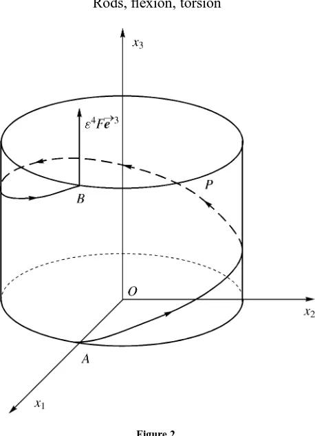
6.2. Example: helicoïdal rod with a free extremity
As mentioned in the introduction, slight modifications of the previous theory allows us to consider other situations, mainly concerning the boundary conditions. We adress here a case where one of the extremities is clamped and the other is free.
We consider the helix defined by
x1=cosθ,
x2=sinθ, 0< θ < π.
Figure 2.
The applied forces reduce to a point forceε4Fe
3applied at the free extremity, where (O;e1,e2,e3)is the frame associated with the cartesian coordinates x1, x2, x3. Moreover, we consider an isotropic homogeneous material, so that the constitutive law is (6.1) with
KI J=
ES 0 0 0
0 EI3 0 0
0 0 EI2 0
0 0 0 E
2(1+ν)I1
, (6.4)
where we recognize the classical coefficients of rigidity for traction, flexions and torsion respectively for the section dilated to the variables z(and consequently independent of ε). This choice allows us to compute the resultant T and the moment M at each point and to work out the problem almost explicitly.
It is well known that the curvaturekand the torsionτ are constant and respectively equal to
k= 1
1+h2, τ=
h
1+h2. (6.5)
Then, from the equilibrium equations (2.1) it follows
ε3 d
ds T
1
a1
+ε4dT
ds + · · · =0⇒T
1
As the given force atB is F=ε4Fe3, we immediatly see thatT1≡0 and we have
The components, in the Frenet frame, of the moment satisfy
from which it follows
d2M2
The componentM2is of the form:
M2(s)=αcos√ s
1+h2 +βsin
s
√ 1+h2. The condition at the free extremity gives
M2 2πp1+h2=0⇒α=0 from which
M2(s)=βsin√ s
1+h2. (6.8)
It immediatly follows
whereβ, C1andC2are arbitrary constants. AsB is free of applied moments
Now, we compute the constantβ: the second Eq. (6.7) gives, on account of the relations (6.10)
dM2
ds 2π
p
1+h2=√ F
From the constitutive law (6.4) withT1
=0,T2
= −M3,T3
=M2,T4
=M1 and using the expressions (5.12) of theEI which are in our case
we obtain the system satisfied by the unknowns u0(s)andθ (s):
which may be written under the matrix form:
d
Using Maple, D. Choï gave the eigenvalues of the matrix, which are
the solution is thus of the form
˜
u0(s)=
4
X
i=1
Ci eλisvi +uf(s),
where the functions vi and uf are easily computed by formal calculus.
Clearly, (6.14) shows that the torsion angle u04(s)≡θ (s) is coupled with the others so that the torsion phenomenon is of the same order as the flexions.
7. General coupled case with given forces of orderε4
We now consider the same problem as in Section 5 in the general case where the local constitutive law involves the tractionT1. We shall also assume that the curvaturekdoes not vanish identically. According to the general properties (see Section 4.1) the traction is of orderε3and the equilibrium equations at that order give
dT1
ds =0⇒T
1
=Const
kT1=0 wherek6=0⇒T1=0
⇒T1=0 everywhere. (7.1)
It then follows that the resultant is, as in Section 5, Tε=ε4T+ · · ·and we shall denote as in Section 4.2 byλ
the first component of T.
In the present case, we have 6 unknowns: u0, θ, E
1, λand also 6 equations: the four Eqs (4.25),T1=0 and the constraint (4.26).
In fact, without using the equilibrium equations, we may obtainT1
=0 from the variational formulation. Indeed, it writes:
Z l
0 4
X
I=1
TIEI∗ds=
Z l
0
fivi+m1θ
ds (7.2)
then, by taking as test element (0,0,0,0, E1∗)with arbitraryE1∗∈L2(0, l), we haveT1 =0,
As a result, the resultant Tε is of orderε4so that the equations and the orders of magnitude are the same as in Section 4, i.e. (4.25). Obviously, the expressions of the functionsEI are the same as in Subsection 5.2.
8. Case when certain given forces are of orderε3
Let us recal that, in Subsection 4.1, we introduced a rather artificial term mε=ε4m1a1(applied moment by unit length). This allowed us to understand better the meaning of the different terms involved in the problem.
Analogously, the problem in Section 7 is not very clear since the unknownE1 is involved in the constutive local law whereas the corresponding forceT1vanishes.
It should also be noticed that
E1= duˆ11
ds −kuˆ
1 2
A better understanding of the problem is obtain when applying, in addition to fεandε4m1a1, a given abstract “force”F ∈L2(0, l)associated withE1. The variational formulation becomes
Z l
0 4
X
I=1
TiE∗I ds=
Z l
0 3
X
i=1
fivi+m1v4+F E1∗
!
ds (8.1)
then, taking the test function(0,0,0,0, E1∗) with arbitraryE1∗∈L2(0, l),we see that (8.1) givesT1=F (which agree with Section 7 whereT1
=0 forF =0).
Let us search for the equations of statics of the present problem. We saw, in Section 4, that the component in G0of the applied forces give a vanishing work for the inextensional displacements. These forces are of the form
g1= −dp
ds, g2= −kp, g3=0,
(8.2)
wherep∈L2(0, l). Let us then consider an auxiliary problem where the applied forces have the form (8.2). The Eqs (2.2) of statics give
T1=p∈L2(0, l).
Consequently, for given applied forces fε=(fε1, fε2, fε3), mε=mε1a1of the form
fε1=ε3
− ddFs
+ε4f1, fε2=ε3(−kF )+ε4f2, fε3=ε4f3,
mε1=ε4m1
withF ∈L2(0, l),f1, m1
∈H−1(0, l),f2, f3
∈H−2(0, l)the equations of the problem are
T1=F (8.3)
with the Eqs (4.25). It will be noticed that
Tε·a1=ε3F +ε4λ+ · · ·, (8.4) whereλis the Lagrange multiplier which appears in (4.25), associated with the inextensibility constraint, and
F is associated with the force g défined by (8.2) withp=F.
References
Alvarez-Dios J.A., Viaño J.M., 1998. Mathematical justification of a one-dimensional model for general elastic shallow arches. Math. Meth. Appl. Sci. 21, 281–325.
Brezzi F., Fortin M., 1991. Mixed and Hybrid Finite Element Methods. Springer.
Chapelle D., 1997. A locking free approximation of curved rods by straigth beam elements. Numer. Math. 77, 299–322. Chenais D., Paumier J.C., 1994. On the locking phenomenon for a class of elliptic problems. Numer. Math. 67, 427–440.
Jamal R., 1998. Modélisation asymptotique des comportements statique et vibratoire des tiges courbes élastiques. Thèse de l’Université Paris VI. Jamal R., Sanchez Palencia É., 1996. Théorie asymptotique des tiges courbes anisotropes. C. R. Acad. Sci. Paris, Ser. I 322, 1099–1106. Lichnerowicz A., 1960. Éléments de calcul tensoriel. Armand Colin, Paris, new edition Jacques Gabay, Paris.
Madani K., 1998. Etude des structures élastiques élancées à rayon de courbure faiblement variable: Une classification des modèles asymptotiques. C. R. Acad. Sci. Paris, Ser. IIb 326, 605–608.
Sanchez-Hubert J., Sanchez Palencia É., 1991. Couplage flexion torsion traction dans les poutres anisotropes à section hétérogènes. C. R. Acad. Sci., Paris, Ser. II, 312, 337–344.