ROOF RECONSTRUCTION FROM AIRBORNE LASER SCANNING DATA BASED ON
IMAGE PROCESSING METHODS
S. Goebbelsa, R. Pohle-Fr¨ohlicha a
Niederrhein University of Applied Sciences, Reinarzstr. 49, 47805 Krefeld, Germany - (Steffen.Goebbels, Regina.Pohle)@hsnr.de
Commission III, WG III/5
KEY WORDS:building modeling, airborne LiDAR, planar faces, CityGML, complex roof structure
ABSTRACT:
The paper presents a new data-driven approach to generate CityGML building models from airborne laser scanning data. The approach is based on image processing methods applied to an interpolated height map and avoids shortcomings of established methods for plane detection like Hough transform or RANSAC algorithms on point clouds. The improvement originates in an interpolation algorithm that generates a height map from sparse point cloud data by preserving ridge lines and step edges of roofs. Roof planes then are detected by clustering the height map’s gradient angles, parameterizations of planes are estimated and used to filter out noise around ridge lines. On that basis, a raster representation of roof facets is generated. Then roof polygons are determined from region outlines, connected to a roof boundary graph, and simplified. Whereas the method is not limited to churches, the method’s performance is primarily tested for church roofs of the German city of Krefeld because of their complexity. To eliminate inaccuracies of spires, contours of towers are detected additionally, and spires are rendered as solids of revolution. In our experiments, the new data-driven method lead to significantly better building models than the previously applied model-driven approach.
1. INTRODUCTION
The German state of North Rhine-Westphalia has published a country-wide city model in CityGML data format, see (Gr¨oger et al., 2012, Kolbe, 2009). In these data, roofs have been recon-structed from sparse point clouds obtained from airborne laser scanning data (LiDAR) by using a model-driven approach, see (Oestereich, 2014). Figures 1, and 3 show the given LiDAR res-olution, which is less then ten points per square meter. The goal of this paper is to improve the quality of this city model with a special focus on buildings with complex roof structures like churches. Among others, applications are solar and shadow im-pact analysis.
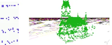
Figure 1: Left picture shows resolution of LiDAR point cloud: Each pixel is of size10cm×10cm, the points are organized in stripes. The right picture displays all points of Luther church.
The literature differentiates between model and data-driven meth-ods (see (Tarsha-Kurdi et al., 2007), cf. (Dorninger and Pfeifer, 2008, Henn et al., 2013, Xiong et al., 2014)): Model-driven meth-ods match the points with standard roof structures taken from a catalogue. This has the advantage that artifacts in point clouds are filtered out, but it has the disadvantage that small structures are generally ignored and atypical roof structures (occurring for example with churches) cannot be matched with roof types from the catalogue. Data-driven methods overcome this problem by fitting single planar facets or other geometric primitives to the point cloud (see e. g. (Elbrink and Vosselman, 2009, Kada and
Wichmann, 2013, Lafarge and Mallet, 2012)). However, data-driven methods are difficult to use for sparse point clouds where details and noise are difficult to distinguish. For a comprehensive overview of both model and data-driven methods see (He, 2015, Henn et al., 2013, Perera and Maas, 2012).
Figure 2: Shortcomings of the existing city model: Most churches are represented in LoD 1. Projection of terrestrial col-ored LiDAR points to facades shows that wall polygons do not fit with facades because of wrong roof angles and missing roof structures.
Our aim is to improve reconstruction of complex roofs in the city model for which the model-driven approach failed to find a Level of Detail 2 (LoD 2) representation or delivers a quality that is not sufficient for automated texture mapping. Especially in the given city model, all churches with complex roofs (like churches in gothic revival style) are only described in LoD 1 by an average height and a ground plan. Also, dormers result in higher walls and wrong roof angles so that real facades differ from the model (see Figure 2). Therefore, we use a data-driven method for im-provement.
transform is very sensitive to noise. Also, we detected planes with high voting values that did not correspond to roof planes. That happens, if a plane intersects with many structures – which, unfortunately, is typical for church roofs.
Region growing based on vector normals, computed byk near-est neighbors, is another near-established method to detect planes, cf. (Rabbani et al., 2006). In our experiments, we got continuous transitions at sharp edges and did not find all areas of roof facets. Surfaces with modest differences in inclination could not be dis-tinguished. There was an effect of leakage at the border of roof facets so that different facets became connected. In addition to that, the method also appeared to be very sensitive to noise. To overcome these problems, the algorithm of (Lafarge and Mallet, 2012) tests the quality of the region growing’s outcome and re-jects poor quality planes and other geometric structures. But then a triangulation is needed to fill gaps.
A RANdom SAmple Consensus (RANSAC) algorithm selects plane parameters from the point cloud and tests them against the data set (cf. (Schnabel et al., 2007, Li et al., 2013)). We tested an M-Estimator SAmple Consensus algorithm that successively estimated planes and removed such points from the cloud that al-ready were allocated to planes. The algorithm wrongly allocated points belonging to other roof segments near intersection lines between planes. Old roof facets are not completely plane. This lead to two or more parallel planes instead of one.
Guided by the disadvantages observed for these established meth-ods, we search for roof facets on a height map that is interpolated from the point cloud instead of directly using sparse cloud data. Interpolation leads to a much denser distribution of points such that not only better and more stable results can be obtained by using previously described methods but also image processing methods can be applied directly to the image that is given by the height map. This fits with a result of (Zebedin et al., 2008) that re-gion growing leads to good results on dense height data obtained from areal images.
Our goal is to keep the original boundary structure of roof facets. Roof polygons often have vertices that are either vertices of the ground plan, intersection points of intersection lines between roof planes or intersection points of these intersection lines with edges of the ground plan. Such roofs are determined by ridge lines so that the basic roof structure can be obtained from intersection lines between planes. However, this is not the complete truth. There might be roof planes that do not intersect within the roof because of step edges. Examples are co-planar planes that occur with shed roofs or roof tops of dormers that may only have one intersection line with the surrounding roof segment. Step edges are discontinuities in a height map, whereas ridge lines are dis-continuities of the height maps’s gradient picture.
Nearest neighbor interpolation, i.e. the use of a Voronoi diagram, does not conserve such boundary structures well. Because of this, Chen et al. introduced a better morphological interpolation method for the case that only a few raster values are missing (Chen et al., 2014). The method works well for the presented test data set that mostly contains flat roofs of high rises. Our data appears to be more complex, and at the same time the height map is filled sparser. Therefore, we use a different interpolation algo-rithm that maintains step edges and does not smudge height in-formation along ridge lines so that noise along ridge lines can be removed later. The algorithm is described in the next section that also covers the detection of facets by clustering similar gradient values of the interpolated height map, as well as the computa-tion of Hesse normal forms of the facets’ planes. Seccomputa-tion 3. then
describes how roof polygons can be derived, simplified and com-bined to an accurate CityGML model. In contrast to the model based algorithm that lead to the North Rhine-Westphalian model, our data-driven approach works without segmentation of build-ings into smaller building parts according to ground plan edges.
We tested our method with geographical data of North Rhine-Westphalia1. It turned out that, for some high towers, there are shadows at one side, where LiDAR data is missing. Also, roof facets of towers tend to be quite small so that normal vectors be-come error prone. Therefore, we handle spires differently.
2. PREPROCESSING OF POINT CLOUD DATA
In this section we describe processing steps for detecting roof facets.
• In a first step we calculate the height map, which we inter-polate from the point cloud.
• We detect roof facets by segmenting angles of gradients of the height map. To this end, we first exclude flat areas. This step is necessary, because the gradient direction for such ar-eas is affected by noise and therefore the analysis of the gra-dient direction does not provide useful information. Outside flat areas, an image of gradient angles is calculated from the height map. With threshold segmentation of angles, areas of roof facets are detected and used for plane estimation.
• Considering missing LiDAR data and non-plane surfaces of tower roofs like cupolas, we also need to estimate the shape of tower roofs in terms of solids of revolution (cf. (Zebedin et al., 2008)).
• With the results of preceding steps, a raster representation of roof facets is generated.
In what follows, the various steps will be described in more detail.
2.1 Interpolation of the height map
Our approach works on a height map in raster domain, where each pixel represents an area of10×10cm2
. This degree of pre-cision appears to be sufficient, because we use LiDAR data with an error of that magnitude. If the points are projected onto the ground plane, the map is only sparsely and non-uniformly filled from the given point cloud. For some regions, data is missing due to shadowing effects (see Figure 3). This holds particularly true for towers or any tower-like roof. Due to the irregular distribution of the points in the cloud, a simple estimation of the height val-ues based on distance weighted mean valval-ues from theknearest neighbors is not possible. In some cases, step edges do not run straightly but obliquely across the roof so that an oblique course as well as jumps also occur in height data (see Figure 4). For correct height estimation, we therefore have to ensure that not only neighbor pixels from one side are taken into account, but rather that opposing neighbors are used for the height interpola-tion. This leads to our algorithm. For each pixel(x0, y0) with unknown height informationz0, we are looking for the pixel’s k = 20 nearest neighbors that belong to the projected point cloud and are below a threshold distance. We need to discuss all possiblek(k−1)/2combinations of two neighbor points. For each pair((x1, y1),(x2, y2))of neighbors, we calculate the
1
cosine value of the angle between vectors(x1 −x0, y1−y0) and(x2−x0, y2−y0)that point from the pixel’s position to the neighbors (scalar product of the normalized vectors). The cosine reaches its minimum−1, if the vectors point exactly in opposite directions. That is the desired situation for interpolation, because all three points lie on a straight line, with the unknown pixel in the middle. Thus, we sort all pairs of two neighbor points according to their cosine value, starting with the smallest. If there is more than one pair with the same cosine value, we additionally sort by the sum of distances
d:=p(x0−x1)2+(y0−y1)2+ p
(x0−x2)2+(y0−y2)2,
starting with the shortest. Following this order, we test, if the pair’s height deviation|z1−z2|is below one meter. If the devi-ation exceeds this limit, we choose the next pair. Otherwise, we determine the missing pixel value by linear interpolation between the heights of the two chosen points(x1, y1, z1)and(x2, y2, z2) (see Figure 5):
z0 :=z1+
(z2−z1) p
(x0−x1)2+ (y0−y1)2
d .
The idea of using symmetrically placed neighbors is not new, see (Otepka et al., 2013) for an overview. For example (Chaudhuri, 1996) defines the barycentric neighborhood, where the distance between neighbors and their centroid becomes as small as possi-ble. However, in our case the centroid is not variable but given by missing pixel data.
Because we only consider points with height deviation below one meter, sharp step edges and correct edge courses are maintained. Figure 4 shows the outcome of our interpolation of the market church in Krefeld-H¨uls. The computation of the height map in raster format now gives us the opportunity to use image process-ing methods in followprocess-ing steps. This is a clear advantage com-pared to other possible approaches.
Figure 3: Points of the top of the tower are missing in the original point cloud of market church.
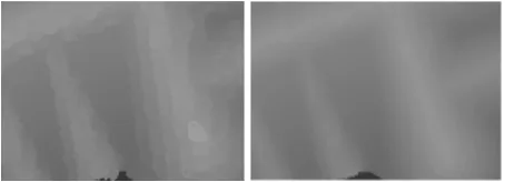
Figure 4: Left: A height map based on the distance weighted mean values from thek nearest neighbors shows stripe-like ar-tifacts that result from irregular distribution of LiDAR points. Right: In a height map generated by our interpolation method, artifacts are eliminated but step edges are maintained.
Figure 5: Selection of pixels used for interpolation in our method, red: the height value of this position has to be computed by in-terpolation, green and blue: 20 nearest neighbors of the red pixel in the point cloud, blue: selected cloud points for interpolation, black: unused cloud points
2.2 Estimation of plane equations for roof facets
Now, we compute the gradient map of the completely filled height map with the Scharr operator which, compared to the Sobel op-erator, better takes rotational symmetry into account. Since the gradient direction in horizontal regions is influenced by noise, we need to handle these regions with small gradient magnitude separately. For all pixel regions with a gradient magnitude lower than a threshold (we used 2 in our implementation), we compute Hesse normal forms (i.e. normal vectors and distances between plane and origin) for the plane with the RANSAC algorithm. For all other regions with higher gradient magnitude, we compute an angle image based on the gradient direction. In the smoothed an-gle histogram, local maxima are determined. The local minima between these maxima are used as threshold values for segmen-tation (see Figure 6). According to these thresholds we divide the angle image into segments that represent roof facets.
In the next step, for each of these segments a Hesse normal form of a plane is estimated with RANSAC algorithm. Planes are ac-cepted, if more than 80 points support the plane model. (Zhou and Neumann, 2012) proposes to use regularities, like opposing projections of normals on the x-y-plane, to adjust roof patch pairs. We also tried to improve the quality of normal vectors by adjust-ing them accordadjust-ing to ground plan edges. But the quality of the estimated Hesse normal forms is so good that we could not find significantly better results with the adjustment.
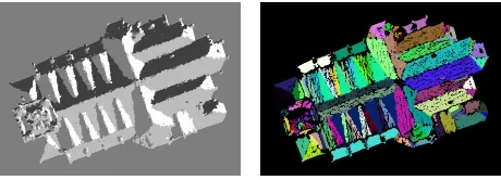
The result of the segmentation process is shown in Figure 7. There, for each roof facet all points that fit with the corresponding plane are drawn with a color that is specific for the facet.
Figure 6: Left picture shows gradient directions computed from the height map. Partial derivatives are displayed as red and green values. The right picture shows a histogram of the gradient an-gles. The histogram is smoothed with a Gaussian filter. Detected maxima and threshold values for segmentation (which are the minima) are marked with lines.
2.3 Tower shape estimation
Figure 7: From left to right: Segmentation result after thresh-olding and points of detected roof facets that fit with the facets estimated plane. Each facet is marked with a different color.
between maximum height value and average height. These re-gions are candidates for towers and will be analyzed further. We identified thresholdh0 experimentally, but it works well for all kinds of buildings, not only for churches. In general we made sure that threshold values are not specific for single buildings so that no manual interaction is required. In our experiments, we accept each region with heights above the threshold as a tower candidate, if it consists of at least 80 pixels. Smaller regions might also stand for other high objects such as trees, antennas or chimneys. But we also have to take the shape of the region into account. Because we work in raster domain, we do not ap-ply established shape indices for polygons involving perimeter (cf. (de Smith et al., 2015, Section 4.2.8)). Instead, we compute the center of gravity(x0, y0)for each candidate region. Then we determine the radiusr0 of the largest enclosed circle with centre(x0, y0)and the radiusR0of the minimal enclosing circle with the same centre. The ratior0/R0is a measure of the tower’s shape. If the tower is perfectly round, this shape index is one. For a rectangular region, where one side has lengthaand the other side is of lengthb, the ratio ismin{a, b}/√a2+b2. Especially if the tower’s ground plan is a square, the ratio is1/√2≈0.71. The more the shape differs from a circle or square, the more un-likely is the candidate region to be a tower. Therefore, we discard all regions with a ratio that is less than 0.5. For example, this excludes rectangular shapes with side lengthsa= 2bfrom being tower candidates.
For each identified tower region, we reconstruct the roof struc-ture within the largest enclosed circle plus an offset of 10 pixels to the radius, giving a radiusR. Within that new circle, we trans-form the height maph(x, y)from Cartesian to polar coordinates ˜
h(r, ϕ) := h(x0+rcos(ϕ), y0+rsin(ϕ)), i.e.˜h(r, ϕ)maps the interval[0, R]×[0,2π)to height values, see Figure 8.
The contour of the spire is defined by the function
f(r) := min{h˜(r, ϕ) :ϕ∈[0,2π)}, (1)
which then is median smoothed and simplified to a piecewise lin-ear curve on[0, R]by applying the Ramer-Douglas-Peucker al-gorithm (Ramer, 1972). Figure 9 shows some results.
We also tried a different approach by computing voting numbers for pairs of radius and height values. To this end, we counted, how often such a combination occurred for all angles ϕk :=
k·2π
n , 0 ≤ k < n, nbeing sufficiently large. By interpreting
voting values as weights, we applied Dijkstra’s shortest path al-gorithm to find another candidate for the tower’s contour. How-ever, this approach lead to similar results as the simpler definition off(r)in (1) so that we did not pursue it further.
To include the circular tower structures into the model, we add a facet on a horizontal plane with height aboveh0as a base. Pix-els within a circle of radius2.5·Raround(x0, y0)are replaced
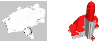
Figure 8: From left to right: Detected tower region in the height map in Cartesian and polar coordinates
Figure 9: Estimated tower shapes in comparison with the original shapes in the point cloud
by pixels of this new facet, if their height exceeds the height of the horizontal plane and if they do not belong to roof facets that reach into the circle from the outside. This is necessary to avoid incomplete structures near the side walls of the tower.
2.4 Filling of gaps and elimination of noise
So far, plane facets have been identified from the interpolated height map in raster domain. Hesse normal forms of the facets’ planes have been computed and points belonging to each facet are marked with a specific color as a unique facet-id in another raster map that now is the base for subsequent computations. In that map, not all raster pixels are covered, and there still is noise around facets’ edges.
Figure 10: A Hough-transform determines step lines going through step edges in the interior of the ground plan.
Ridge lines are pieces of intersection lines between the planes that are defined via Hesse normal forms. Only those pieces of step lines and intersection lines are relevant, where there are pix-els in the neighborhood that have significant height differences or belong to facets of both intersecting planes.
To avoid influence of noise near step lines and ridge lines, we remove colored pixels that are closer than half a meter to a rele-vant piece of a line, if they are not connected to other pixels of that color which are farer away from the line and placed on the same side of the line. Then we iteratively let the pixels inside the ground plan grow until they collide or until a step line or an intersection line belonging to the pixel’s plane is reached, or un-til the interpolated height of the next pixel differs more than a threshold value from the current one. If there are still blank areas after this step, then we repeat it without considering intersection lines or step edges. Along this procedure, facets might become unconnected. Such facets have to be split up into separate con-nected components to allow computations that are described in the next section. Intermediate and final results of the filling pro-cess are shown in Figures 11 (cf. Figure 7) and 12 for market (H¨ulser Kirche) and main church (Dionysiuskirche).
Figure 11: Processing for the market church in Figure 7 contin-ued: The upper left picture shows the ground plan, bold cyan intersection lines between planes and thin violet step lines (spire has been removed). The upper right picture displays the result of filling with respect to intersection lines and step edges. The lower left figure shows the outcome of polygon detection and simplifi-cation. Also, the final 3D model of the market church is shown.
3. COMPUTATION OF ROOF POLYGONS
3.1 Construction of roof polygons
To cope with openings, we partially sort the list of roof facets such that each facet is completely surrounded at most by facets that are later in the list. Following this order, one can compute outer polygons on the basis that inner polygons have been deter-mined already.
Following the topological order iteratively, for each facet we per-form these steps:
• We execute Pavlidis’ algorithm (see (Pavlidis, 1982, Chap-ter 10)) to find an ordered list of vertices of the ouChap-ter bound-ary polygon of the facet. The applied version of the algo-rithm moves along the facet’s raster map border in a clock-wise fashion.
Figure 12: Starting with a raster map of pixels allocated to planes, we repeat the processing steps shown in Figure 11 for the main church of the town.
• For each vertex, we determine a list of adjacent facets from colors of pixels in the neighborhood to the left side of the vertex according to the direction of Pavlidis’ algorithm, see Figure 13. Pixels to the right have to be ignored, especially if the local width of the current facet only is one pixel. Oth-erwise, one would find neighbor facets in a wrong order. For implementation, we divide each pixel into four sub-pixels, move from sub-pixel to sub-pixel and use a 4-neighborhood of sub-pixels to find the left-sided adjacent facets.
Because of the topological order of facets, each detected boundary vertex belongs at most to outer (and not to inner) boundaries of those of the facets that have been dealt with previously.
• There might be sections of the polygon that define a com-mon outer border with facets of previous iterations or with the ground plan of the building. These sections of vertices can be easily identified by vertices’ list of adjacent facets. The sections have to be joined with corresponding vertex se-quences of the previously computed outer border polygons or with vertex sequences of the ground plan. The outcome is a boundary graph that defines the roof topology. This is nec-essary to generate a ”waterproof” model without gaps be-tween different roof facets. It is helpful that the construction ensures common vertex sequences to be previously stored in an order opposite to the order in which they are visited by Pavlidis’ algorithm for the current facet (cf. directions in Figure 13).
The boundary graph has to be simplified by removing vertices with the Ramer-Douglas-Peucker algorithm from (Ramer, 1972). In addition to the original algorithm, we maintain the position of those vertices, where segments of different facets are joined. Such vertices represent the topological structure of the roof. Also, the positions of vertices of the ground plan are kept.
So far, precision is limited to the10×10cm2
Figure 13: Each pixel is divided into 4 sub-pixels. The arrows show steps of Pavlidis’ algorithm. Only the blue pixel is neighbor of the sub-pixel that is marked with a cross. The cross touches all neigbors of a 4-neighborhood of sub-pixels.
raster representation. In order to remove remaining noise and to get a building that precisely fits with the ground plan from cadastral data, we snap vertices according to distance threshold values (see Table 1) to each other, to vertices of the ground plan and to intersection points of intersection lines between planes, if a plausibility check regarding heights succeeds. Also, we only snap vertices to intersection points if they have at least two adjacent facets in common. Additionally, we project vertices onto near edges of the ground plan. A vertex might also be projected onto a near intersection line between planes, if the intersecting planes belong to the facets that are adjacent to the vertex. Throughout all these operations, we do not modify ground plan vertices and do not move intersection points. Figures 11 and 12 show resulting roof layouts.
max. deviation for Ramer-Douglas-Peucker alg. 1 m
min. vertex distance 30 cm
max. distance for snapping to ground plan edges 30 cm snapping to intersection points within 60 cm projection to ground plan edges if nearer than 30 cm projection to related intersection lines if nearer 40 cm
Table 1: Threshold values for polygon simplification and merging
3.2 CityGML generation
Finally, we generate a CityGML representation of the building. Heights of roof vertices are computed using Hesse normal forms of corresponding roof planes. In general, by projecting vertices to intersection lines, we avoid the model to have step edges where ridge lines should be. However, roof facets of old buildings might not be absolutely plane, and we miss small facets. Therefore, there might be height deviations at vertices where more than two facets intersect. To eliminate these deviations, we compute sep-arate height values for each vertex with respect to Hesse normal forms of all adjacent roof facets. We group the height values into classes with widths of at most a configurable threshold value. When drawing a roof facet, for each vertex we select the class that contains the height value of this facet. Then we draw the vertex with an weighted average of heights of this class. Weights are taken from facets’ pixel counts. In our test data set a threshold of 0.5m works well with a few exceptions,1.3m eliminates erro-neous step edges completely. Unfortunately, polygons based on averaged heights do only define an approximately planar geom-etry. If seen strictly, this violates a CityGML requirement. We do not cure this problem by post processing, because roof poly-gons in the given North Rhine-Westphalian city model are also not exactly planar due to rounding errors of similar magnitude. In general, a triangulation of roof facets is needed to draw them. If one uses the same normal vector for lighting of all triangles, small deviations are not visible.
Also, polygons of spires are generated from contour data (cf. Sec-tion 2.3) by dividing representative disks into segments. Using a
principle component analysis, the polygonal base of each spire is rotated such that the orientation of the edges fits with the build-ing’s orientation.
The CityGML terrain intersection polygon is the ground plan from cadastral data enriched with heights from airborne laser scanning. Attributes like address, number of floors or building’s usage are taken from cadastral data.
A roof facet that completely surrounds another facet, can be mod-eled as a LoD 3 roof surface. In CityGML, LoD 2 surfaces do not allow for openings. However, if the inner roof facet completely lies above the outer roof segment, then we do not model the LoD 3 opening in the outer facet but use a simpler LoD 2 structure to increase drawing performance. Typically, this is the case for dormers.
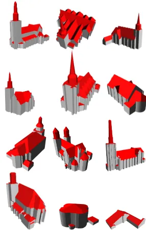
Figure 21 shows a collection of church models that are generated by our algorithm.
4. EVALUATION
Since no ground truth of surface planes was available for the city of Krefeld, we measured the accuracy of 63 church models by considering all LiDAR points(x, y, z)for which(x, y)lay within the ground plan. For each point we calculated the absolute dif-ference|z−h(x, y)|, whereh(x, y)denotes the model’s height above position(x, y)as determined by the correspondig plane’s estimated Hesse normal form. Spires are drawn with plane tri-angles. To get error numbers that are independent of the number of vertical segments used for triangulation, we instead computed heights of the original, non-triangulated solid of revolution de-fined by the piecewise linear contour that is described in Section 2.3. Figure 14 summarizes arithmetic means, standard deviation and median of absolute differences. If one takes into account that we work on a 10 cm raster with threshold values of Table 1, the overall accuracy appears to be surprisingly good, especially the median values are nearly optimal. Arithmetic means show much larger errors because of the influence of high towers. Significant deviations mostly occurred in the neighborhood of step edges and towers, see Figure 15.
There are a couple of reasons for systematic errors. Whereas the given LiDAR data covers chimneys and antennas, these structures are not included in the model. We handle spires as described in Section 2.3 which is the reason for larger deviations than we get for other roof structures. Especially, we have to incorporate plateaus as bases for solids of revolution,
Another problem is that LiDAR points belonging to trees were not filtered out. If such points did not influence roof plane de-tection, the correct result was measured as an error, because we wrongly compared with LiDAR points of trees. On the other hand side, some trees were mistaken for roof planes, see Figure 16. The error measure does not cover this type of problem. It also does not show that our building models are limited to the area in-side the ground plan taken from cadastral data. Therefore, roofs are cut off at ground plan edges, some canopies are missing.
Figure 14: Accuracy for each church (numbered 1–61) in metres: The upper diagram shows median value of absolute differences between model and point cloud, the lower diagram shows arith-metic mean and standard deviation.
Figure 15: Pictures show error map and model of the church with the largest error.
5. FUTURE WORK
In future, we will differentiate between different tower shapes such as round or square towers. This can be done by interpreting the height map at a constant distance from the center of gravity (x0, y0). Significant height values were found for the half radius R/2, cf. Section 2.3. Towers with square shapes show typical curved signatures depending on the number of corners, whereas round towers show a smooth line signature. The analysis of the type of signature is possible by means of Fourier transform or by considering the number and positions of local extrema.
Cupolas outside tower areas should be identified using pattern recognition methods. We are investigating techniques to model dormers and small tower-like structures. A further improvement would be to extend roof facets to areas outside the ground plan according to LiDAR data. On the other hand side, as shown in (Zebedin et al., 2008), instead of just applying a Ramer-Douglas-Peucker-type algorithm to simplify polygons locally, it is
pos-Figure 16: Trees around the left church lead to three small towers at corners of the building. Because of the same reason, the right church has an error at the left front side.
Figure 17: Central station: model-driven (left) and data-driven approach (right). In the model-driven approach, the tower was mistaken as a roof.
sible to generate various level of geometric detail using global optimization.
6. CONCLUSIONS
Resolution of public laser scanning data of North Rhine-West-phalia is sufficiently precise to create LoD 2 models of churches and buildings with non-standard roof structures. Our data-driven method yields better results than the previously used model-dri-ven method. The quality of the models is adequate for automated mapping of photographs to facades.
REFERENCES
Chaudhuri, B., 1996. A new definition of neighborhood of a point in multi-dimensional space. Pattern Recognit. Lett. 17, pp. 11– 17.
Chen, Y., Cheng, L., Li, M., Wang, J., Tong, L. and Yang, K., 2014. Multiscale grid method for detection and reconstruction of building roofs from airborne lidar data. IEEE J. Sel. Topics Appl. Earth Observ. Remote Sens. 7(10), pp. 4081–4094.
de Smith, M. J., Goodchild, M. F. and Longley, P. A., 2015. Geospatial Analysis. Fifth edn, The Winchelsea Press.
Dorninger, P. and Pfeifer, N., 2008. A comprehensive automated 3d approach for building extraction, reconstruction, and regular-ization from airborne laser scanning point clouds. Sensors 8(11), pp. 7323–7343.
Elbrink, S. O. and Vosselman, G., 2009. Building reconstruction by target based graph matching on incomplete laser data: analysis and limitations. Sensors 9(8), pp. 6101–6118.
Figure 19: A projection of terrestrial colored LiDAR points onto walls within a maximum distance of three meters shows differ-ences between the existing model-driven (tower missing) and the new data-driven method. There are points missing at tower walls (grey color) because they were partially hidden from the scanner. White points mark errors.
Figure 20: Johannes church in a city model context and in reality
Gr¨oger, G., Kolbe, T. H., Nagel, C. and H¨afele, K. H., 2012. OpenGIS City Geography Markup Language (CityGML) Encod-ing Standard. Version 2.0.0. Open Geospatial Consortium.
He, Y., 2015. Automated 3D Building Modeling from Airborne LiDAR Data (PhD thesis). University of Melbourne, Melbourne.
Henn, A., Gr¨oger, G., Stroh, V. and Pl¨umer, L., 2013. Model driven reconstruction of roofs from sparse lidar point clouds. IS-PRS Journal of Photogrammetry and Remote Sensing 76, pp. 17– 29.
Huang, H. and Brenner, C., 2011. Rule-based roof plane detec-tion and segmentadetec-tion from laser point clouds. In: Joint Urban Remote Sensing Event (JURSE), 2011, pp. 293–296.
Kada, M. and Wichmann, A., 2013. Feature-driven 3d building modeling using planar halfspaces. ISPRS Ann. Photogramm. Re-mote Sens. and Spatial Inf. Sci. II-3/W3, pp. 37–42.
Kolbe, H., 2009. Representing and exchanging 3d city models with citygml. In: J. Lee and S. Ziatanova (eds), Representing and Exchanging 3D City Models with CityGML, Lecture Notes in Geoinformation and Cartography, Springer, Berlin, pp. 15–31.
Lafarge, F. and Mallet, C., 2012. Creating large-scale city models from 3d-point clouds: A robust approach with hybrid representa-tion. International Journal of Computer Vision 99(1), pp. 69–85.
Li, J., Xiao, Y. and Wang, C., 2013. Quality assessment of build-ing roof segmentation from airborne lidar data. In: 21st Interna-tional Conference on Geoinformatics 2013, pp. 1–4.
Oestereich, M., 2014. Das 3D-Geb¨audemodell im Level of Detail 2 des Landes NRW. Nachrichten aus dem ¨offentlichen Vermes-sungswesen Nordrhein-Westfalen 47(1), pp. 7–13.
Otepka, J., Ghuffar, S., Waldhauser, C., Hochreiter, R. and Pfeifer, N., 2013. Georeferenced point clouds: a survey of fea-tures and point cloud management. ISPRS Int. J. Geo-Inf. 2, pp. 1038–1065.
Overby, J., Bodum, L., Kjems, E. and Ilsøe, P. M., 2004. Au-tomatic 3d building reconstruction from airborne laser scanning data using hough transform. International Archives of Pho-togrammetry and Remote Sensing 35(B3), pp. 296–301.
Figure 21: A collection of data-driven church models
Pavlidis, T., 1982. Algorithms for Graphics and Image Process-ing. Springer, Berlin.
Perera, S. N. and Maas, N. G., 2012. A topology based approach for the generation and regularization of roof outlines in airborne laser scanning data. DGPF Tagungsband 21, pp. 1–10.
Rabbani, T., van den Heuvel, F. and Vosselmann, G., 2006. Seg-mentation of point clouds using smoothness constraint. Interna-tional Archives of Photogrammetry, Remote Sensing and Spatial Information Sciences 36(5), pp. 248–253.
Ramer, U., 1972. An iterative procedure for the polygonal ap-proximation of plane curves. Computer Graphics and Image Pro-cessing 1(3), pp. 244–256.
Sampath, A. and Shan, J., 2010. Segmentation and reconstruction of polyhedral building roofs from arial lidar point clouds. IEEE Trans. Geosci. Remote Sens. 48(3), pp. 1554–1567.
Schnabel, R., Wahl, R. and Klein, R., 2007. Ransac based out-of-core point-cloud shape detection for city-modeling. Schriften-reihe des DVW, Terrestrisches Laser-Scanning (TLS 2007).
Tarsha-Kurdi, F., Landes, T., Grussenmeyer, P. and Koehl, M., 2007. Model-driven and data-driven approaches using lidar data: Analysis and comparison. International Archives of Pho-togrammetry, Remote Sensing and Spatial Information Sciences 36(3/W49A), pp. 87–92.
Xiong, B., Elberink, S. O. and Vosselman, G., 2014. Building modeling from noisy photogrammetric point clouds. ISPRS Ann. Photogramm. Remote Sens. and Spatial Inf. Sci. II-3, pp. 197– 204.
Zebedin, L., Bauer, J., Karner, K. and Bischof, H., 2008. Fusion of feature- and area-based information for urban buildings mod-eling from aerial imagery. In: Computer Vision – ECCV 2008, Lecture Notes in Computer Science 5305, pp. 873–886.