Valuing groundwater recharge through agricultural production in the
Hadejia-Nguru wetlands in northern Nigeria
Gayatri Acharya
a,∗, Edward B. Barbier
baEnvironmental Economist, The World Bank, 1818 H Street, Washington DC 20433, USA bReader, Environment Department, University of York, Heslington, York YO1, 5DD, UK
Received 5 May 1998; received in revised form 10 November 1999; accepted 24 November 1999
Abstract
This study applies a production function approach to value the groundwater recharge function of the Hadejia-Nguru wetlands in northern Nigeria. The groundwater recharge function supports dry season agricultural production which is dependent on groundwater abstraction for irrigation. Using survey data this paper first carries out an economic valuation of agricultural production, per hectare of irrigated land. We then value the recharge function as an environmental input into the dry season agricultural production and derive appropriate welfare change measures. Welfare change is calculated using the estimated production functions and hypothetical changes in groundwater recharge and hence, groundwater levels. By focusing on agricultural production dependent solely on groundwater resources from the shallow aquifer, this study establishes that the groundwater recharge function of the wetlands is of significant importance for the floodplain. © 2000 Elsevier Science B.V. All rights reserved.
JEL classification: Q10; Q25
Keywords: Production function approach; Valuation; Wetlands; Groundwater recharge; Ecosystem function
1. Introduction
The Hadejia-Nguru wetlands in northern Nigeria are formed by the floodwaters of the region’s two prin-cipal rivers, the Hadejia and the Jama’are. The rivers exhibit ephemeral flow patterns with periods of no flow in the dry season (October–April). Almost 80% of the total annual runoff occurs in August/September. (Thompson and Hollis, 1995). During this period, wa-terlogged areas known as fadamas are formed and are
∗Corresponding author. Tel.:+1-202-458-9545;
fax:+1-202-676-0977.
E-mail address: [email protected] (G. Acharya)
important not only for fishing and agricultural activi-ties, making these some of the most productive areas in northern Nigeria, but also for providing recharge to the underlying aquifers (Hollis and Thompson, 1993). Water from these aquifers is used for domestic con-sumption and for irrigation during the dry season.
A number of water diversion schemes have been constructed or are planned upstream of these wet-lands. These schemes will divert floodwater away from the wetlands, reducing the annual flooding within the floodplain (Hollis et al., 1993). Barbier et al., (1993) and Barbier and Thompson (1998) have shown that the economic value of the wetlands in terms of floodplain agriculture and fishing, is
icant and will be affected by the construction of new dams and water diversion schemes. The economic value of the opportunity costs associated with divert-ing this water away from the wetlands has not been fully realised and incorporated into the development plans for this region. Hydrologists have noted that an important environmental function of these wetlands is in recharging the groundwater resources of the area (DIYAM, 1987; Thompson and Hollis, 1995).
The aim of this paper is to partially value the groundwater recharge function of the wetlands by ap-plying the production function approach to analysing groundwater use in irrigated agriculture.1 The groundwater recharge function is assumed to sup-port dry season agricultural production dependent on groundwater abstraction for irrigation. Using sur-vey data on agricultural production in the floodplain, this paper first carries out an economic valuation of agricultural production, per hectare of irrigated land. Following approaches advocated in the valuation liter-ature (Ellis and Fisher, 1987; Mäler, 1992; Freeman, 1993; Barbier, 1994), we value the recharge function (through water input) as an environmental input in dry season agricultural production dependent solely on groundwater resources from the shallow aquifer. Two welfare change measures are derived and related to the recharge function of the wetland. Welfare change is then calculated using the estimated production func-tions and hypothetical changes in groundwater level.
2. Groundwater use in irrigated dry season farming
Agriculture in the Hadejia-Jama’are floodplain in-volves both dryland and fadama farming. These areas are flooded during the wet season and gradually dry out until they are flooded again during the next wet season. Floodplain activities have adapted to make use of the floodwaters and the fadamas in an ingenious way, taking advantage of the wetland’s resources for grazing, agriculture and other economic uses.
1Throughout this paper, irrigated agriculture refers to irrigation with groundwater pumped up from the shallow aquifer with the use of small tubewells. Domestic water consumption within the wetlands is also dependent on groundwater resources, see Acharya (1998).
Total cultivated area in the floodplain is estimated as 230,000 ha (Barbier et al., 1993). Upland or dry-land farming is rain-fed, and millet, sorghum and cow-melon are cultivated. Fadama farming is mainly rice cultivation. In addition, there are irrigated lands where vegetables may be grown during the dry sea-son. The three main types of irrigation technologies used in this area are identified by Adams (1993) as ditch irrigation, shadoof irrigation and pump irriga-tion. This study focuses on pump irrigation using wa-ter from shallow aquifers. Irrigation farming begins in October, after the floods have receded, and continues up until March/April. The floodplain has experienced a dramatic rise in small-scale irrigation following the introduction of small petrol powered pumps for sur-face water irrigation and tubewells to tap the shallow aquifers under the floodplain (Kimmage and Adams, 1992; Kaigama and Omeje, 1994). Although the extent of small scale tubewell irrigation within the Hadejia-Jama’are wetlands is not well documented, changes in hydrological conditions, economic con-ditions, government initiatives, and in particular the policies of World Bank supported Agricultural Devel-opment Programs (ADPs) have promoted the use of small irrigation pumps through subsidies and/or loans for tubewell drilling and pump purchase. DIYAM (1987) suggests that shallow aquifers could irrigate 19,000 ha within the wetlands through the use of these small tubewells. NEAZDP (1994) suggests that the annual increase in cropped area within the wetlands is at least 10% and could be higher in areas where water and suitable land is available.
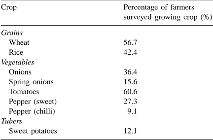
Table 1
Main commercial crops cultivated
Crop Percentage of farmers
surveyed growing crop (%)
Grains
Wheat 56.7
Rice 42.4
Vegetables
Onions 36.4
Spring onions 15.6
Tomatoes 60.6
Pepper (sweet) 27.3
Pepper (chilli) 9.1
Tubers
Sweet potatoes 12.1
this area is generally subsistence and to hedge against uncertainty farmers practice multi-cropping and inter-cropping. Farmers are, therefore, mainly subsistence oriented agricultural households, also producing cash crops.
3. Economic valuation of dry season irrigated agriculture
Production data on crops grown in the study area are based on the results of field surveys carried out in four villages in the Madachi fadama from November 1995–March 1996. The villages of Madachi, Ando, Alaye and Maluri are believed to be representative of the villages in the wetlands, comprising a range of large, medium and small farmers. A total of 37 farms were surveyed for crop production data. In addition, the entire influence area of the Madachi fadama was surveyed to establish the number of operational tubewells in the area and a total of 309 operational tubewells were counted during this survey period (HNWCP, 1996). Wheat, tomatoes and pepper are the main cash crops being cultivated in the study area (Table 1). Okra and eggplant (the latter is grown in large quantities where there is surface irrigation) are also grown but mainly for home consumption and in small quantities.
The total area of small scale irrigation using ground-water resources within the Madachi fadama and its influence area is estimated to be around 66 km2, or
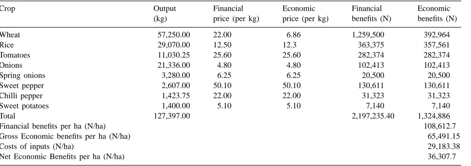
ap-proximately 6600 ha.2 The value of the output from the farms surveyed as shown in Table 2. Financial prices for the outputs are estimated from market sur-veys conducted between December 1995 and May 1996 and from survey findings of farmgate prices re-ceived by farmers. Outputs are based on harvest fig-ures reported in sacks or bundles by farmers and con-verted to weight measures, based on results from the market survey.
The per hectare value for irrigated agriculture in the Madachi area is 36,308 Naira or US$ 412.5 per hectare. The economic value of dry season irrigated agriculture from the Madachi fadama influence area (6600 ha) is estimated as 2.39×10⁸ Naira or US$ 2,723,077.3
4. The production function approach and crop-water relationships
This section develops the underlying general wel-fare estimation theory based on the production func-tion approach (see Mäler, 1992; Freeman, 1993; Barbier, 1994). The specific production functions for wheat and vegetables based on the production and input data collected by the survey are estimated in Section 5. Based on this analysis and the production functions, welfare estimates related to a change in water input are calculated in Section 6.
4.1. Production function approach
We begin by assuming that farmers produce I=1,
. . ., n crops, irrigated by groundwater. Let yi be the
aggregate output of the ith rop produced by the farm-ers. The production of yi requires a water input Wi,
2 This figure is based on Thompson and Goes (1997) which states that the influence area of the Madachi fadama may be estimated as 136 km2, assuming a minimum of 1 km radius of influence. The largest extent of the actual swamp area has been estimated as 78 km2and we estimate an area of 66 km2as being serviced by the recharge from the fadama and as being available for agricultural activities.
Table 2
Economic valuation of irrigated agriculture for survey villages (area: 20.23 ha)a
Crop Output Financial Economic Financial Economic
(kg) price (per kg) price (per kg) benefits (N) benefits (N)
Wheat 57,250.00 22.00 6.86 1,259,500 392,964
Rice 29,070.00 12.50 12.3 363,375 357,561
Tomatoes 11,030.25 25.60 25.60 282,374 282,374
Onions 21,336.00 4.80 4.80 102,413 102,413
Spring onions 3,280.00 6.25 6.25 20,500 20,500
Sweet pepper 2,607.00 50.10 50.10 130,611 130,611
Chilli pepper 1,423.75 22.00 22.00 31,323 31,323
Sweet potatoes 1,400.00 5.10 5.10 7,140 7,140
Total 127,397.00 2,197,235.40 1,324,886
Financial benefits per ha (N/ha) 108,612.7
Gross Economic benefits per ha (N/ha) 65,491.15
Costs of inputs (N/ha) 29,183.38
Net Economic Benefits per ha (N/ha) 36,307.7
aExchange rate N88=$1.
abstracted through shallow tubewells, and j=1,. . ., J of other variable inputs (e.g. fertilisers, seed, labour), which we denote as xi,. . ., xJor in vector form asXXXJ.
Because of the relationship between recharge and the level of water in the aquifer, we also assume that the amount of water available to the farmer for abstraction is dependent on the groundwater level, R. The aggre-gate production function for crop i can be expressed as:
yi =yi(xi1. . . xij, Wi(R)) for alli (1)
and the associated costs of producing yi are:
Ci =CCCxXXXJ +cW(R)Wi for alli (2)
where Ci is the minimum costs associated with
pro-ducing yi during a single growing season, cw is the
cost of pumping water andCCCxis a vector ofcxi. . . cxJ
strictly positive, input prices associated with the vari-able inputsxi1. . . xiJ. Note that we assume cw is an
increasing function of the groundwater level, R, to allow for the possibility of increased pumping costs from greater depths, i.e.c′W >0, c′′W>0. We first
assume that there exists an inverse demand curve for the aggregate crop output, yi:
Pi =Pi(yi) for alli (3)
where Pi is the market price for yi, and all other
marketed input prices are assumed constant.
Denoting Si as the social welfare arising from
pro-ducing yi, Siis measured as the area under the demand
curve (3), less the cost of the inputs used in produc-tion4:
Si=Si(xi1, . . . xiJ, Wi(R);cw(R))
=
Z y1
0
Pi(u)du−CCCxXXXJ−cw(R)Wi for alli, j (4)
To maximise (4) we find the optimal values of input
xiJ and water input Wi through setting the following
first order conditions to zero:
∂Si ∂xiJ
=Pi(yi) ∂yi ∂xiJ
−cxJ =0 for alli, j (5)
∂Si ∂Wi
=Pi(yi) ∂yi ∂Wi
−cw(R)=0 for alli (6)
Eqs. (5) and (6) are the standard optimality conditions indicating that the socially efficient level of input use occurs where the value of the marginal product of each input equals its price. If each farmer is a price-taker, then this welfare optimum is also the competitive equi-librium. We assume that this is the case.
The first order conditions in (5) and (6) can be used to define optimal input demand functions for all other inputs as xiJ∗ = xiJ∗(cxJ, cw(R), R) and
for water as Wi∗ = Wi∗(cxJ, cw(R), R). In turn, the
optimal production and welfare functions are de-fined as y∗i = y∗i(xi∗, . . . , xj∗, Wj∗(R)) and Si∗ =
Si∗(xiJ∗, . . . , xiJ∗, WJ∗(R);cw(R)).5
From the above relationships, we are interested in solving explicitly for the effects on social wel-fare of a change in groundwater levels, R, due to a fall in recharge rates. Assuming that all other inputs are held constant at their optimal levels, and that all input and output prices (with the exception of cw)
are unchanged, it follows from the envelope theorem that:
The net welfare change is, therefore, the effect of a change in groundwater levels on the value of the marginal product of water in production, less the per unit cost of a change in water input. The marginal change in pumping costs also affects the total costs of water pumped (Wi∗(∂cw/∂R)). The effect of a change
in water input due to a change in groundwater levels occurs both directly(∂W/∂R)and indirectly through the marginal effect of a change in pumping costs on water input ((∂Wi/∂cw)(∂cw/∂R)). As long as per
unit pumping costs are not prohibitively high, one would expect an increase in groundwater levels (to a point) to lead to a welfare benefit, or at least to main-tain the initial welfare levels, whereas a decrease in groundwater levels would result in a welfare loss, either due to increased pumping costs and/or change in productivity.
If we now assume that all farmers face the same production and cost relationships (1) and (2) for each crop i and are price takers, then it is possible to derive the aggregate welfare effects of a non-marginal change in groundwater levels. Let there be 1, . . ., k farmers producing yik output of crop i and using wik water
inputs. It follows that by integrating (7) over R0 (old
level) to R1(new level) and aggregating across all K 5Asterisks denote optimally chosen quantities.
farmers yields the welfare effects of a no-marginal change in groundwater levels on the aggregate output of crop i.
Implementing the above welfare measure in (8) re-quires knowledge of the production function for each crop, as well as how the equilibrium output and in-puts change with R. Alternatively, we could measure the aggregate welfare effects directly from changes in social welfare, Si, in Eq. (4) above. This would
imply:
where y0is the initial output level and y1is the final
output level. To use (9) as a welfare measure we would also need to estimate production functions for each crop and calculate optimal levels of inputs and out-puts. We return to these welfare measures in Section 6 where, using the information from estimated pro-duction functions, we use both measures to calculate welfare change for our sample of wheat and vegetable farmers.
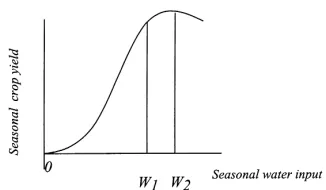
4.2. Irrigation inputs and crop yields
availability; climatic factors such as evaporation rates; soil factors, including soil type and soil moisture and the length of the growing period. Fig. 1 below depicts seasonal crop response to variable water input show-ing zones of increasshow-ing returns (0,W), diminishshow-ing returns (W1,W2) and negative returns (>W2).
Various functional forms have been used in the lit-erature to describe production technologies using data from field experiments and from observed farm data. The simplest conception of crop response to water application is the linear response and is most likely when the range of application of the variable inputs is small. Log-linear relationships using Cobb–Douglas production functions have also been used to estimate crop-water relationships, although a maximum prod-uct is not defined by the Cobb–Douglas and conse-quently, a decreasing total product (e.g. at high levels of water application) is not possible. A polynomial function such as a quadratic or Gompertz function would allow estimation of the effect of increasing in-put levels and diminishing marginal returns, as would a Cobb–Douglas translog function, particularly when a wider range of inputs are considered (Hexem and Heady, 1978; Carruthers and Clark, 1981).6 The survey data used here contains information on ac-tual quantities and market prices of inputs used and yields. It therefore reflects optimisation behaviour on the part of the farmers and is more than a physical relationship between the inputs it reflects economic
6Crop-input functions such as Mitscherlich–Spillman functions are often used to estimate effects of changes in water input, given that the application of all other inputs remain constant. These functional forms obey the von Liebig law of the minimum which asserts that there may be non-substitution between some nutrients and a yield plateau. Mitscherlich proposed an exponential functional form specified as:
yi=m(1−ke−β2i)
where yi is the observed yield and ai is the growth factor of the crop. m is defined as the asymptotic yield plateau. The Von Liebig function assumes that output increases linearly in the input up to some maximum. These functional forms have been used with experimental data to study the input-crop production relationship. Experimental data would need to be generated to find the maximum for each input. Yield and output data generated by these agronomic experiments do not, however, reflect optimising behaviour and we use market generated and farm data for the production function estimation.
Fig. 1. Crop-water relationships (adapted from Carruthers and Clark, 1981).
Fig. 2. Water pumping costs as a function of water table depth.
decisions as well. Hence, production functions for the crops are estimated using the survey data.7
Before estimating production functions and welfare changes we also consider the technological relation-ship between groundwater levels and tubewells. A typ-ical tubewell consists of a length of pipe pump casing sunk into the ground below the maximum depth to the water table. This maximum depth should be such that during pumping, the aquifer’s water level does not fall below the pipe’s reach. If the rate of withdrawal from
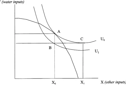
Fig. 3. Effect of a non-marginal change in water table depth on the production possibilities frontier.
the aquifer exceeds the recharge, and groundwater lev-els do not recover to the original base level, the use of the shallow tubewell will need to be abandoned.8
For the purpose of this study, there are two possible effects of a fall in groundwater levels:
(i) as groundwater falls below a certain level, the costs of pumping water are likely to rise, and (ii) if groundwater levels fall below the maximum
depth of the sunken tubewells, the farmer will cease pumping for the rest of the dry season and agricul-tural production will fall.
Fig. 2 describes the effect of changing groundwa-ter levels on the marginal costs of pumping wagroundwa-ter and Fig. 3 depicts the effect of changing groundwater lev-els on the farmer’s production possibilities frontier. Water inputs are denoted by W and other inputs by X, while R denotes groundwater levels.
The tubewells in the study area are sunk to depths of approximately 9 m. This implies that the groundwa-ter table would have to fall to a level greagroundwa-ter than 9 m (Rsin Fig. 2) before pumping capabilities fall to zero,
i.e. for case (ii) to occur. If this occurs, and assum-ing that all other inputs are held constant, the farmer normally producing at Point A (W0,X0) is forced to
operate at Point B, defined by (W1,X0) in Fig. 3. The 8However, increased costs of pumping from a greater depth may cause pumping to be curtailed until a new groundwater level is established. Because the farmer is forced to stop pumping, water levels may recover, allowing some sporadic pumping throughout the season. This introduces uncertainty into the problem and makes it a dynamic problem. This is beyond the scope of the present paper.
farmer’s production possibilities frontier (PPF) moves in because of a fall in depth beyond 9 m. He cannot maintain his original level of utility and move to Point C at (W1,X1) because this point lies outside the
pro-duction possibilities frontier (since the farmer cannot change input decisions during the season). The farmer will, therefore, operate at Point B and produce a lower output, or not produce at all.9 At Rs, the
disconti-nuity that sets in due to technological limitations, in effect drives the cost of pumping water to infinity for the farmer. This non-convexity in the cost curve may be offset by technological innovation. However, given the present level of technology, if the water levels stay below 9 m, the farmer will not be able to irrigate at all and the associated drop in yield can be calculated from the production function by setting water input to zero. This is only expected to occur in the wetlands if there is a long period of very low flooding and no technological change.
For case (i) to occur, we expect that the speed of the pump will be affected by a drop in groundwater levels but water will still be available to the farmer using the given technology. The pumps being used in the flood-plain are surface mounted pumps, and it is likely that at depths approaching 7 m (denoted as R1 in Fig. 2),
these pumps will slow down because of the increase in lift. To maintain input levels, the farmer would have to increase pumping hours, thereby incurring higher costs of production (C1). However, the farmer may be
able to continue production in the short run. Using the data on pumping hours and the specifications of the pumps being used, we estimate that as water levels drop from 6 m to 7 m, pump speeds will decrease from 37,636 l/h to 26,434 l/h (approximately 30% decrease in speed).10
We use this information to calculate the unit pump-ing cost at the new groundwater level, R2. As Fig. 2
shows, Cw(R)=C0for levels of R≤R0. Pumping costs
increase thereafter. By linearising the cost function be-tween R0 and R1 in Fig. 3, we derive the functional
relationship between pumping costs, cw and
ground-water level R for R0≤R≤R1as:
cW(R)=a+bR (10)
where a=−19.56; b=5.34.
Note that this functional form, with the values for
a and b as noted above, only describes the portion
of the curve between R0 and R1 in Fig. 2. We can
estimate the change in pumping costs due to a fall in groundwater levels using the above relationship and the welfare measure in (9). Increases in pumping costs will also affect the level of water input during the growing season and optimal levels of water input and associated change in output levels can be calculated from the production functions, estimated in Section 5, and the optimality conditions in (5) and (6).
5. Estimating production functions for wheat and vegetables
In the production functions estimated below, we as-sume that output (y) depends on land (L), labour (B), Seeds (S), fertiliser (F) and water inputs (W). The farmers in the Madachi area mainly grow wheat,
irri-10Although, theoretically per unit costs of pumping water should be constant for the given technology, surface mounted pumps are less efficient at groundwater depths approaching 7 m. If costs are constant the welfare change for the farmer would be measured by:
dSi dR =
Z R1
R0
Pi(yi∗) ∂yi ∂Wi −cw
∂Wi ∂R
dR
gated rice and vegetables. The crops are divided into these three groups because of the different nature of irrigation, fertiliser application and other farming de-cisions. Wheat and rice are generally grown earlier in the season and vegetables are grown well into the dry season. In the following sections, we estimate pro-duction relationships for wheat and vegetables only since irrigated rice is grown by very few farmers in the sample.11
We consider linear and log-linear functional forms for wheat and vegetable production.12 The linear form assumes constant marginal products and excludes any interaction between the inputs. Although the lack of interaction terms is restrictive, we observe in the litera-ture that linear relationships are likely, particularly for wheat production and with low levels of inputs. The log-linear form assumes constant input elasticities and variable marginal products. Note that the coefficients estimated by using this form represent output elastici-ties of individual variables and the sum of these elas-ticities indicates the nature of returns to scale. Table 3 lists the variables used in the analysis. The estimated linear and log-linear production functions for wheat are:
Y =α+β1L+β2B+β3S+β4F +β5W+ε1(11)
lnY=α+β1lnL+β2B+β3lnS
+β4lnF +β5lnW+ε2 (12)
andεi is the random disturbance associated with the
production function.
The production function for vegetables was also es-timated as a single function since all the vegetables
11Since crop level data is often not available, many studies analyse farm level aggregated input demands. Although fixed factors, such as land, may cause jointness in the production process, we argue that crop level production functions can be estimated in this case for wheat and for vegetables since (1) crop level data was collected through the survey and is available and (2) vegetables are clearly grown only after the winter wheat production implying that input decisions may be considered as separate in terms of the production processes.
Table 3
Table of variable names
Variable Definition
Y Output (kg)
L Land (ha)
B Labour (workers)
F Fertiliser (kg)
S Seeds (kg)
W Water (l)
LY LN (Y)
LL LN (Land)
LB LN(Labour)
LF LN (Fertiliser)
LS LN(Seeds)
LW LN(Water)
are grown at the same time (after the wheat has been harvested) or in quick succession and receive simi-lar quantities of inputs. Data on seeds/seedlings (S) was unreliable and this variable was dropped from the above estimated production functions (11) and (12) for vegetables.
Table 4 reports the results for the linear and log-linear functions for wheat production. The linear model has an R2of 0.93 and F statistic of 54.4. Both the values suggest a good fit. The Breusch–Pagan La-grange Multiplier test is not significant for the linear model (critical value for LMχ2=13.27; with 5 d.f.),
Table 4
Results for the wheat production functiona
Variable Linear Log-linear
Land 1993.7b (2.865) –
Labour (B) 52.711 (0.824) –
Seeds 3.6165c (2.566) –
Fertiliser 71.581c (2.438) –
Water 11.610c (2.134) –
LL – 0.38 (1.442)
LB – −0.024 (0.156)
LS – 0.026 (0.33)
LF – 0.47b(2.71)
LW – 0.6885d(1.881)
Constant −1662.5b(3.598) 3.4c(2.39)
Adjusted R2 0.93 0.9
F statistic 54.4 37.49
Breusch–Paganχ2 1.05 (d.f.5) 18.27 (d.f.5)
Observations 21 21
at statistics in parenthesis. b2% significance level. c5% significance level. d10% significance level.
and we accept the hypothesis of homoscedasticity. However, the large, negatively signed and statistically significant value for the constant term would suggest that there might be misspecification of the functional form.
The log-linear functional form also performs well in terms of R2(0.9) and F statistics (37.49). The co-efficients for LW and LF are found to be statistically significant in the log-linear model, with the expected signs. The Lagrange multiplier statistic is however significant for the log-linear model, indicating some heteroscedasticity in this model. The presence of this heteroscedasticity indicates that the least squares es-timators are still unbiased but inefficient. Since the estimators of the variances are also biased we cor-rect for the standard errors of the coefficients and find relatively small differences in the values. The log-linear model is, therefore, considered as the most satisfactory version of the wheat production function. According to the literature on crop-water produc-tion funcproduc-tions determined from experimental studies, wheat is often seen to have a linear or log-linear shape unlike other crops which may show diminishing re-turns at high levels of water application. Wheat may continue to show increasing returns up to fairly high levels of water application (Hexem and Heady, 1978; Carruthers and Clark, 1981).
Table 5 reports the econometric results for the func-tions estimation for vegetable production. The linear
Table 5
Results for the vegetable production functiona
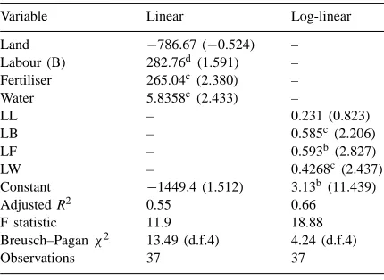
Variable Linear Log-linear
Land −786.67 (−0.524) – Labour (B) 282.76d (1.591) – Fertiliser 265.04c (2.380) –
Water 5.8358c (2.433) –
LL – 0.231 (0.823)
LB – 0.585c(2.206)
LF – 0.593b (2.827)
LW – 0.4268c(2.437)
Constant −1449.4 (1.512) 3.13b (11.439)
Adjusted R2 0.55 0.66
F statistic 11.9 18.88
Breusch–Paganχ2 13.49 (d.f.4) 4.24 (d.f.4)
Observations 37 37
and log-linear models again perform well in terms of R2and F statistics. The Breusch–Pagan Lagrange Multiplier test is significant for the linear model (χ2=13.49; with 4 d.f.), and we reject the hypothesis of homoscedasticity. For the log-linear model, the Lagrange multiplier statistic is less than the critical value at the 5% significance level (χ2=4.24; with 4 d.f.), indicating no heteroscedasticity in this model. The coefficients on the variables LF, LB, LW and the constant term are statistically significant.
6. Valuing the recharge function
Hydrological evidence for the relationship be-tween flood extent and recharge to village wells show that there is some fluctuation with flood extent and mean water depth of the shallow aquifer. The ef-fect of planned upstream water projects will have an impact on producer welfare within the wetlands through changes in flood extent therefore groundwater recharge. By hypothesising a drop in groundwater lev-els from 6 m to 7 m in depth (due to reduced recharge in the current period), we calculate the expected change in welfare associated with this reduction in recharge. This exogenous change affects the farmers decision making process during the farming season, i.e. after decisions on other inputs have already been taken since the effect of the reduced recharge will not be felt until after the dry season agriculture has started.
Recall that in Section 4.1, the welfare change mea-sure for non-marginal changes in R (level of naturally recharged groundwater) is given by (8). This welfare change measure is used together with the results of the production function estimates to calculate welfare changes for individual farmers. We also assume that farmers in the Madachi area are price takers and hence face a ‘horizontal’ demand function, i.e. Pi(yi)=Pi.
From Eq. (8) we see that the effect of R on wel-fare is felt through a change in water input due to in-creased costs ((∂Wi/∂cw)) and/or a change in water
availability(∂Wi/∂R). This second effect will occur
only if a change in recharge were to cause a decline in groundwater levels below 9 m (see Section 4.2 and Fig. 3 above). This is unlikely to happen within a sin-gle season and we do not therefore consider this aspect in calculating welfare change. Instead we consider the
effect of changing pumping costs on water input and use the production function estimated earlier for the purpose of estimating welfare changes. However, in order to do so, we need to calculate(∂Wi/∂cw), the
marginal change in water demand due to a marginal change in the cost of pumping.
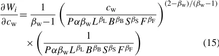
In Section 5 we estimated production functions for wheat and vegetable production. Holding all other in-puts constant and noting that only water input will vary, we use the log linear production functions esti-mated in Section 5, together with the optimality con-ditions in Eqs. (5) and (6) to solve for Wi as:
PiαβWLβLBβBSβSFβFWβW−1=cw (13)
Wi∗= cw
PiαβwjLβLBβBSβSFβF
!1/(βwi−1)
(14)
where L,B, S and F are all the other inputs in the specified production function (for crop i) with esti-mated parameters βL, βB, βS and βF.13 We solve
for(∂Wi/∂cw)as: ∂Wi
∂cw
= 1
βw−1
c
w
P αβwLβLBβBSβSFβF
(2−βw)/(βw−1)
×
1
P αβwLβLBβBSβSFβF
(15)
This is calculated for each farmer, using the estimated values for the relevant parameters and constant terms and the market price of the crop.
We now calculate welfare change due to a drop in groundwater levels to 7 m, for individual farmers, us-ing the welfare measures in Eq. (8) or Eq. (9) (see Appendix A for the derivation of expressions used to calculate welfare changes). The production functions from Section 5 are used to calculate the associated change in productivity due to a fall in recharge lev-els. We calculate optimal levels of water input from (13) and output levels from the production function. The average and total change in welfare for a drop in groundwater levels from 6 to 7 m depth, using both welfare measures (8) and (9), are given below. From (8), the welfare change of a drop in groundwater lev-els (R) to 7 m is calculated as given in Table 6. From
Table 6
Welfare change for sample using Eq. (8)
Crop Total welfare change (Naira) Average welfare change per hectare Total land (ha) Average land holding (ha)
Wheat 551,201 54,459 10.51 0.645
Vegetables 105,916 3,566 29.7 0.803
Table 7
Welfare changes for sample using Eq. (9)
Crop Total welfare change (Naira) Average welfare change per hectare Total land (ha) Average land holding (ha)
Wheat 550,320 54,372 10.51 0.645
Vegetables 130,659 4,399 29.7 0.803
(9), the welfare change of a drop in groundwater lev-els (R) to 7 m is calculated as in Table 7.
As expected, there is only a small variation between the results from using the two welfare change mea-sures. The welfare change associated with the effects of groundwater loss on wheat production is very high. Although vegetable production is, in general, more water intensive, it appears that wheat production is more sensitive to changes in water input. The elastic-ity of production to water inputs for wheat is higher than it is in the case of vegetable production. However, vegetable production takes place well into the dry sea-son and may be subject to even higher pumping costs for water if the water table falls below 7 m during the dry season. To properly measure this welfare change we would, however, require knowledge of the full re-lationship between pumping costs and groundwater levels. Since there is little evidence that groundwater levels could fall much below 7 m we have restricted our present analysis to this level for both wheat and vegetable production.
The Madachi fadama affects an area of about 6600 ha. Although there are at least 963 tubewells installed in the area, only 309 were found to be cur-rently operational (i.e. 32% of installed tubewells are
Table 8
Welfare change in the Madachi fadama in Nairaa
Average welfare change per farmer Total loss for Madachi farmers
Vegetable farmer 2,863 383,642
Wheat+vegetable farmer 29,110 5,094,296
aExchange rate: 88 N=US$ 1.
operational). Approximately 56.7% of the farmers in this area grow wheat while 100% of the farmers grow vegetables. This implies that 56.7% of the farmers would be affected by the welfare change associated with growing wheat and vegetables and 43.3% would be affected by the welfare change associated with growing vegetables only. We assume there are a cor-responding number of farmers for each of the 309 operational tubewells and conclude that there are 175 wheat and vegetable farmers and 134 vegetable farm-ers in the Madachi fadama influence area. We use the welfare change measures for a fall in groundwa-ter levels from 6 to 7 m depth from Eq. (9) for the welfare changes reported in Table 8.
veg-etable farmers and 77% of yearly income for vegveg-etable and wheat farmers. The total loss associated with the 1 m change in naturally recharged groundwater lev-els (resulting in a decline of groundwater levlev-els to approximately 7 m) is estimated as 5,477,938 Naira (US$ 62,249) for the influence area of the Madachi
fadama.
The welfare estimates for wheat are surprisingly high. It is argued that the reason for this is that wheat is a newly introduced crop within the wetlands and because of its recent introduction displays a high yield response to water inputs. Since our data is collected over a single dry season, this is reflected in our re-sults. Continued production of wheat within the wet-lands could be subject to declining yields over time and is generally considered to be unsustainable within the wetlands over the long run (Barbier et al., 1994). Disregarding wheat production the estimated welfare loss is therefore 383,642 Naira or US$ 4360 for the study area.
DIYAM (1987) suggested that shallow aquifers could irrigate 19,000 ha within the wetlands through the use of small tubewells. Using the average wel-fare change for the study area of 5478 Naira/ha or US$ 62/ha, we estimate a welfare loss of 1.04×10⁸
Naira or US$ 1,182,737 for the wetlands, due to a decrease in groundwater levels to approximately 7 m in depth.14 Again disregarding wheat production, the welfare loss associated with this change in groundwa-ter levels, amounts to 82,832 US$ for the wetlands. Although there is considerable difference in the level of welfare loss with and without consideration of wheat production, the value of groundwater recharge in terms of irrigated agriculture is clearly positive and significantly large.
7. Conclusions and policy implications
The emphasis on increasing tubewell irrigation within the wetlands is contradictory to policies such as dam construction and channelization that would reduce flooding within the wetlands. The economic
14Note that this figure is based on the percentage of installed tubewells actually working during the study period (32%) and could be much higher for a higher percentage of operational tubewells within the wetlands.
value of the opportunity costs associated with divert-ing this water away from the wetlands has not been fully realised and incorporated into the development plans for this region. Although there is at present apparently little concern for the over-exploitation of groundwater resources, this optimism is based on relatively little data on aquifer recharge and the effect of increased or reduced flooding of fadama areas. Cropping patterns in the area have changed due to credit and technological facilities as well as due to changing hydrological conditions. Increasing dependence on small-scale irrigation for dry season crops may also result in increased sensitivity of small farmers to changes in prices and market demand. As previous studies have asserted, and as this study confirms, groundwater recharge is of considerable im-portance to wetland agriculture and reduced recharge resulting in lower levels of groundwater will result in high welfare losses for the floodplain populations. Furthermore, this analysis has been conducted in the Madachi fadama, a regularly inundated area with good groundwater stocks. It is very likely that in other areas of the wetlands where flooding is not as reliable as in Madachi, the effects of reduced recharge and rapid declines in groundwater levels will have more devastating effects.
unsustainable developments within the wetlands, can-not be ruled out. In the face of this uncertainty, the value of the shallow aquifers in irrigated agriculture, and consequently the value of the recharge function of the wetlands, must be recognised by policies affecting hydrological conditions within the floodplain.
Appendix
Specifically, for each farmer the expression used in calculating welfare change from (9) is:
(SR1)−(SR0)=(Piy1−CCCxXXX∗j−cw(R1)Wi∗(R1))
−(Piy0+CCCxXXX∗j+cw(R0)Wi∗(R0))
We use optimal values for water input levels, eval-uated at the different unit costs of pumping c1 and
c0, assuming all other inputs remain constant.
Opti-mal levels of output, y1 and y0, are then calculated for each farmer at the estimated optimal water input levels. Similarly, we integrate Eq. (8) over R, deriving the following expression:
Evaluating for R=[6,7], we derive the following expression:
Acharya, G., 1998. Hydrological-economic linkages in water resource management. Ph.D. dissertation, University of York (unpublished).
Adams, W.M., 1993. Agriculture, grazing and forestry. In: Hollis, G.E., Adams, W.M., Aminu-Kano, M. (Eds.), The Hadejia-Nguru Wetlands: Environment, Economy and Sustainable Development of a Sahelian Floodplain Wetland, IUCN Gland.
Barbier, E.B., Thompson, J.R., 1998. The value of water: floodplain versus large-scale irrigation benefits in Northern Nigeria. Ambio 27 (6), 434–443.
Barbier, E.B., 1994. Valuing environmental functions: tropical wetlands. Land Econ. 70 (2), 155–173.
Barbier, E.B., Adams, W., Kimmage, K., 1993. Economic valuation of wetland benefits. In: Hollis et al. (Eds.), The Hadejia-Nguru Wetlands. IUCN, Gland
Carruthers, I., Clark, C., 1981. The Economics Of Irrigation. Liverpool University Press, Liverpool.
DIYAM, 1987. Shallow aquifer study, 3 Volumes. Kano State Agricultural and Rural Development Authority, Kano. Ellis, G., Fisher, A., 1987. Valuing the environment as an input.
J. Environ. Manage. (25), 149–156.
Freeman, A.M. 1993. The measurement of environmental and resource values: theory and methods. Resources for the Future, Washington DC.
Hexem, R., Heady, E., 1978. Water Production Functions for Irrigated Agriculture. State University Press, AMES, IO. HNWCP, 1996. Internal report prepared on the survey of
the Madachi fadama influence area. Hadejia-Nguru Wetlands Conservation Project, Nguru.
Hollis, G.E., Adams, W.M., Aminu-Kano, M., (Eds.), 1993. The Hadejia-Nguru Wetlands. IUCN Gland, Cambridge, UK. Hollis, G.E., Thompson, J.R., 1993. Water resource developments
and their hydrological impacts. In: Hollis, G.E., Adams, W.M., Aminu-Kano, M. (Eds.), 1993. The Hadejia-Nguru Wetlands. IUCN Gland, Cambridge, UK.
Mäler, K.G., 1992. Production Function Approach in Developing Countries in Vincent, J.R., Crawford, E.W., Hoehn, J.P. (Eds.) Valuing Environmental Benefits in Developing Countries. Special report 29, Michigan State University, East Lansing. NEAZDP, 1994. Groundwater report. North East Arid Zone
Development Programme (NEAZDP), Gashua, Nigeria. Thompson, J.R., Hollis, G., 1995. Hydrological modelling and
the sustainable development of the Hadejia-Nguru Wetlands, Nigeria. Hydrol. Sci. J. 40, 97–116.