CRITICAL ASSESSMENT OF CORRECTION METHODS FOR FISHEYE LENS
DISTORTION
Y. Liua, C. Tiana, Y. Huanga,∗
a
School of Remote Sensing and Information Engineering, Wuhan University, 129 Luoyu Rd, Wuhan, China, 430079 -(Liuyangyang912, Tianchengshuo1273, hycwhu)@whu.edu.cn
Commission I, WG I/3
KEY WORDS:Fisheye Lens Distortion, Camera Calibration,Critical Assessment
ABSTRACT:
A fisheye lens is widely used to create a wide panoramic or hemispherical image. It is an ultra wide-angle lens that produces strong visual distortion. The distortion modeling and estimation of the fisheye lens are the crucial step for fisheye lens calibration and image rectification in computer vision and close-range photography. There are two kinds of distortion: radial and tangential distortion. Radial distortion is large for fisheye imaging and critical for the subsequent image processing. Although many researchers have developed calibration algorithms of radial distortion of fisheye lens, quantitative evaluation of the correction performance has remained a challenge. This is the first paper that intuitively and objectively evaluates the performance of five different calibration algorithms. Up-to-date research on fisheye lens calibration is comprehensively reviewed to identify the research need. To differentiate their performance in terms of precision and ease-using, five methods are then tested using a diverse set of actual images of the checkerboard that are taken at Wuhan University, China under varying lighting conditions, shadows, and shooting angles. The method of rational function model, which was generally used for wide-angle lens correction, outperforms the other methods. However, the one parameter division model is easy for practical use without compromising too much the precision. The reason is that it depends on the linear structure in the image and requires no preceding calibration. It is a tradeoff between correction precision and ease-using. By critically assessing the strengths and limitations of the existing algorithms, the paper provides valuable insight and guideline for future practice and algorithm development that are important for fisheye lens calibration. It is promising for the optimal design of lens correction models that are suitable for the millions of portable imaging devices.
1. INTRODUCTION
With the development of computer technology, non-metric cam-era has been more widely used in the field of photogrammetry and computer vision. Fisheye lens has a wide field of view up to 180 degree. Because of its remarkable range of view, it is widely ap-plied in the field of military, surveillance, street maps, panorama stitching and so on. However, due to the special imaging process of fisheye lens, the distortion is a main obstacle for practical use. The traditional pinhole model is no longer able to meet the need of fisheye lens correction. We need to consider more parameters and introduce different distortion models for different lens.
Distortion has been researched for many years, and it was first introduced by Conrady in 1919. Following his work, Brown (D-uane, 1971) proposed the radial distortion, tangential distortion and thin prism distortion model which has been widely used for image distortion. On the basis of previous work, some different distortion models are proposed. Zhang (Zhang, 2000) proposed a flexible technique for estimation of radial distortion, which only required the camera to observe a checkerboard from a few dif-ferent orientations, and the method is widely applied because of its easy implement. Fitzgibbon(Fitzgibbon, 2001) showed how to use the division model to solve the problem of nonlinear lens dis-tortion, and Miguel Alem´an-Flores (Alem´an-Flores et al., 2014) then extended the division model. In this model, they combined hough space with the division model, and a single fisheye lens im-age can be corrected without any attached condition. Devernay
∗Corresponding author
and Faugeras (Devernay and Faugeras, 2001) proposed the field-of view(FOV) model and perform edge extraction and polygo-nal approximation. Claus (Claus and Fitzgibbon, 2005) proposed the rational function model and built a general distortion model for large field-of-view lens. Carlos (Ricolfe-Viala and S´anchez-Salmer´on, 2010b) introduced a robust metric calibration. In their paper, they proposed using cross-ratio constraint which is inde-pendent of perspective projection as a template for calibration, so that we can get two sets of point: the distorted points and the corrected points. Zhu (Zhu et al., 2011)proposed a lifting strategy based on an elliptical model for the correction of fish-eye image. Lee (Lee et al., 2011) introduced another method for wide-angle distortion correction with hough transform and gra-dient estimation. There are also other methods,such as virtual grid (Arfaoui and Thibault, 2013), parabolic perspective projec-tion (Zhang, 2012), vanishing point (Hughes et al., 2010) and so on.
the straight line. The count of each bin in the Hough space then represents the degree of correction. The larger the count is, the more feature points are corrected for the line associated with that bin.
The paper is divided as follows. First, brief descriptions of five different distortion models are given. Second, lens calibration via cross-ratio constraint is briefly described. Third, we propose a Hough-based measure for evaluating distortion model. Finally, experimental results and conclusions are presented.
2. FIVE DISTORTION MODELS
The distortion model is a mapping from the distorted image to the corrected image, which is mathematically formulated according to the internal geometry of camera lens. The traditional pinhole model is a ideal model without taking lens distortion into account. The 3-D space points can be transformed to image coordinates with only the intrinsic and external parameters. However, the distortion is inevitable especially for wide-angle lens. Therefore there are various models proposed to solve the distortion and to refine the transformation. Some model are metric methods and other not. In the paper, we compare five metric distortion models according to their popularity and relevance in the state of the art.
2.1 Rational and Tangential Model(RT Model)
Radial and tangential distortion model is a conventional model which is widely accepted. According to the model, the formula of the model takes into account the radial, tangential and prism distortion. Given one point(ud, vd)in the image, its
correspond-ing corrected point(u, v)can be given such that
u=ud−δu(u, v)
v=vd−δv(u, v)
(1)
whereuandvrepresent the undistorted image coordinates, name-ly the ideal position in the image;udandvdare the corresponding
observed points with distortion;δu(u, v)andδv(u, v)are the
dis-tortion inuandvdirection respectively, which is the sum of three types of distortion: the radial, tangential, and prism distortion. It can be written by the following equation:
δu(u, v) =∆ud·(k1·r
drepresents the distance from the image
point to the distortion center, which can be defined as(u0, v0), so
∆ud=ud−u0,∆vd=vd−v0.
The radial distortion is modeled by the first part of the formula. It can be given by
position in the direction ofuandvrespectively. The coefficients k1,k2,k3,...represent the degree of the polynomial function, and
usually the first and the second radial symmetric distortion pa-rameterk1,k2are dominant and others negligible.
The tangential distortion is also known as decentering distortion, which arises from the decentering of lens. This is modeled can
be recorded as
wherep1, p2represent the coefficients of tangential distortion.
Another kind of distortion is called the prism distortion which comes from the tilt of lens when the lens are not perpendicular to the optical axis, and it is modeled bys1, s2. Usually, the radial
distortion is in a dominant position, and the prism distortion is relatively insignificant and can be negligible(Weng et al., 1992).
2.2 Logarithmic Fish-Eye Model(FET Model)
Basu and Licardie (Basu and Licardie, 1995) proposed a alterna-tive model fitting for fisheye lens, which based on the logarith-mic fisheye transformation. Given a point(u, v)representing the distortion-free cartesian coordinates in the image, we can denote (r, θ)as the corresponding polar coordinates, sor=√u2+v2,
θ = arctan(v/u). Then the corresponding distorted polar coor-dinates(rd, θ∗)can be given by
rd=slog(1 +λr), θ∗=θ (5)
whererdis the distorted radius,srepresents the scale factor andλ
controls the amount of distortion over the whole image. Then the corresponding distorted cartesian coordinates(ud, vd)are given
by
ud=rdcosθ∗, vd=rdsinθ∗ (6)
The inverse mapping is given by
rd=
2.3 Polynomial Distortion Model(PFET Model)
The model is one of the most frequently used distortion model, and it is similar to the FET model except thatrd=G(r), where
r is the radial distance for a undistorted image,rdis the distorted
one. It can be given by the following equation:
G(r) =a0+a1r+a2r
wherekrepresents the degree of polynomial function. What is the difference between the polynomial distortion model and the FET model is thatG(r)is a polynomial inr.
2.4 Division Model
Fitzgibbon (Fitzgibbon, 2001) introduced the division model for the simultaneous estimation of multiple view geometry and lens distortion.The division model is written as follows:
p= 1
(1 +λ||x||2) (9)
or can be recorded as
L(r) = 1
(1 +k1r2+k2r4+· · ·)
(10)
d(ud, vd) =
remarkable advantage of this model is that we can correct severe distortion using fewer terms than the polynomial model. Thus, it is more suitable for wide-angle lens. Additionally, the inversion of one parameter division model is simple and can find the roots of a second degree polynomial, so for most camera lens, a single parameter division model is adequate.
2.5 Rational Function Model(RF Model)
To adapt to the imaging process of perspective and non-perspective imaging system, Grossberg(Grossberg and Nayar, 2001) present-ed a general image model which uspresent-ed a set of virtual sensing elements to express the mapping from the incoming scene rays to the physical imaging sensors. It considers the camera as a ”black box” and ignores the concrete process that the light goes through the camera internal optical sensors. Following this idea, Claus and Fitzgibbon(Claus and Fitzgibbon, 2005) extended im-age plane to 3-D scene, and built a general model for highly dis-torted lens, which called the rational function model. Given a distorted image point(ud, vd)and corresponding distortion-free
point(u, v), the mapping can be formulated by the quadratic giv-en by Equation 11. This model can be writtgiv-en as a linear com-bination of the distortion parameters, in3×6matrix A, and a six-vectorx, of monomials inudandvd. Definexas the follows:
x(ud, vd) = [u2d ud·vd v2d ud vd 1]T (12)
So the rational function can be written by
d(ud, vd) =A·x(ud, vd) (13)
wheredis a vector in camera coordinates representing the ray direction along which pixel(ud, vd)samples. So we can have
the perspective projection to obtain the undistorted image coordi-nates. i.e.,
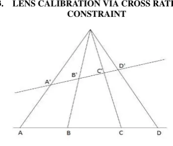
3. LENS CALIBRATION VIA CROSS RATIO CONSTRAINT
Figure 1: Principle of cross-ratio invariablity
According to the perspective projection in Euclidean space, s-traight lines have to be ss-traight after perspective projection. More
details can be found in (Devernay and Faugeras, 2001). In geom-etry, cross ratio remains invariable when they are under perspec-tive projection, as is demonstrated in Figure 1.
Given four points A, B, C, D which lies in a straight line, the cross radio of four co-linear points can be written as
CR(A, B, C, D) = AC CB
AD
DB (15)
where the points A and B are two datum points, and the points C and D are the reference points. When the four point are under perspective projection, there are four corresponding pointsA′, B′,C′,D′in the space. The cross ratio of the new four points
According to projective geometry, if four points are co-linear, the corresponding points also lie on a straight line. Furthermore, the cross ratio is a projective invariant, so that we can conclude that cross ratio of two sets of points is equal, the equation is defined as
In our experiment, we use a checkerboard as a calibration plane, and it is projected on the screen. The corner points are detected on the image, and because of the collinearity of points, the cross ratio should be invariable in the image. Based on the work of Carlos and Antonio-Jose (Ricolfe-Viala and S´anchez-Salmer´on, 2010b) (Ricolfe-Viala and Sanchez-Salmeron, 2010a) who proposed the metric point correction via the cross-ratio constraint, we detected m×ncorner points from the image of the chessboard, wheren is the number of the straight lines in the chessboard pattern and mis the number of points in each line. So,qk,lis a pointkof the
straight linel,l = 1. . . n,k = 1. . . m. To find the coordinate of the distortion-free point corresponding to each distorted point qk,l in the image, the difference of cross-ratio between the four
sets of points detected in the image and the distortion-free ones must be minimized. On the other hand, a point in the straight lines have to fit the linear equation. Therefore, the equation including the two constraints can be given such that
JCP=
line, which represent the linear constraint in the image; the sec-ond part of the equation represents the cross-ratio constraint, and CR(p1, p2, p3, p4)is computed previously which is equal to all
four sets of points in the designed planar template.
in the image and the corresponding distortion-free points via the cross-ratio and linear constraint, we can utilize the set of point pairs to get the coefficients of the five distortion models previ-ously proposed in the paper.
4. HOUGH-BASED MEASURE FOR EVALUATING DISTORTION MODEL
As is mentioned before, there are many fisheye lens calibration methods. Which one is better needs to be determined. Tradition-al evTradition-aluation measure uses error function to represent cTradition-alibration precision, but different models have different error functions. It is difficult to measure them under the unified framework. Be-sides, the error functions is not intuitive. So, a simple but effec-tive evaluation measure is needed. Due to the fact that a line on the distorted image must be corrected into a straight line on the undistorted image, so whether lines of the undistorted image are still straight or not is a good measure of the correction perfor-mance. We analyse these lines in the Hough space, in which one line of the undistorted image is represented by one point (ρ,θ).
Figure 2: Hough transform
ρ=x·cosθ+y·sinθ (19)
whereρis the distance from the origin pointOto the linel. The origin pointO is the top left corner of the undistorted image, andθ is the intersection angle between the line normal and x-coordinate. The x-coordinate and y-coordinate coincide with the column and row on the undistorted image. Equation 19 denotes the coordinate transformation from image space to hough space.
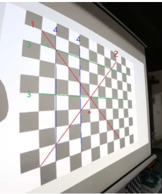
Based on the corner points of the straight lines of the chessboard image, the Hough statistics is made for different (ρ,θ) combina-tions. A large value of the statistical result represents that more points coincide with the same line of (ρ,θ). The line (ρ,θ) of maximal statistical count in the Hough space is found to locate the corner points that are nearly aligned with the most significant line of (ρ,θ) in the image space. By analyzing the statistical consistence of co-linear feature points at different directions in the Hough space, as shown in Figure 3, we can conclude how many points lie in a straight line and how close they are to the straight line. The count of each bin in the Hough space then rep-resents the degree of correction. The larger the count is, the more feature points are corrected for the line associated with that bin.
Evaluation measure consists of two aspects, precision and ease-using. For precision, we analyse the overall and local perfor-mance of lens correction. In the overall analysis, all corner points are checked whether they align with each other; in the local anal-ysis, only lines of a certain direction is checked to evaluate the correction performance at that direction. Calculating the ratio of
Figure 3: Four directions for evaluating lens correction (⊕ repre-sents distortion center)
the aligned points after correction and the total points at a di-rection can evaluate the degree of cordi-rection of different mod-els. High ratio is considered to have a better correction effect. For ease-using, little human interaction without compromising the correction performance is welcomed.
5. EXPERIMENTAL RESULTS
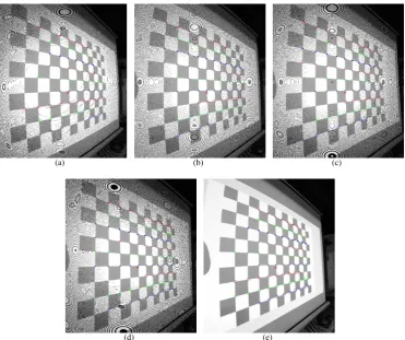
In this section, five fisheye lens calibration models have been test-ed with a diverse set of data which is capturtest-ed by the Canon 5DI-II camera and the fisheye lens of a fixed focal length of 8mm. A chessboard pattern is projected to a large screen by a projec-tor, and taken at Wuhan University, China under varying lighting conditions, shadows, and shooting angles, as the Figure 4 shows. The pattern is made of 10×12 grids, and 99 corner points. The distortion coefficients are obtained by the cross-ratio constraint, which are used to correct the distorted image.
Figure 4: Distorted image captured by fisheye lens with fixed focal length
Table 3: Performance at the direction of 3 and 4
Model Points in direction 3 far to distortion center
Points in direction 3 near to distortion center
Points in direction 4 far to distortion center
Points in direction 4 near to distortion center
RT 8/11 10/11 5/9 7/9
FET 10/11 11/11 6/9 9/9
PFET 10/11 11/11 6/9 9/9
RF 11/11 11/11 9/9 9/9
Div 10/11 11/11 7/9 9/9
are obtained byfindChessboardCorners()andcornerSubPix()of OpenCV3.0. Due to the quantization and rounding error, some of the corrected points may fall outside of the range or be approx-imated. It results in the black points in the corrected image, for which no distorted points are corresponded exactly. But it has no effect on this paper because we aim at addressing the param-eters of different models. With the model paramparam-eters, instead of finding the undistorted point for each distorted point, we can in-versely find the distorted point for each undistorted point by the numerical iteration or interpolation.
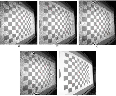
The corner points on the red line of Figure 5 are mapped into the Hough space, where theρstep is set to 14 pixel and theθstep is set to 1 degree. For eachθ, one correspondingρis calculated to get a (ρ,θ) bin in the Hough space.
Based on the statistical count of Hough space, the red line of Figure 5 are located at the bin of (ρ,θ) as follows: (178,41) in RT model with the count number of 5, (179,38) in FET model of number 6, (179,38) in PFET model of number 6, (180,41) in division model of number 7, (180,40) in RF model of number 9. It can be seen that the corrected line varies a little with different correction models. The Hough-based statistics exactly reflects the difference.
The distance threshold that defines whether a corner point is aligned with the line is set to 6 pixels. The lines of different directions in Figure 3 are chosen to evaluate the correction performance of d-ifferent models along dd-ifferent directions. The result of corrected corner points at different directions is demonstrated in Figure 6, Figure 7 and Figure 8.
For traditional RT model, totally 72 corner points are got on al-l al-lines in direction 3 (horizontaal-l direction) and totaal-lal-ly 80 corner points on all lines in direction 4 (vertical direction), as shown in Figure 3. The total points is the least whether seen from hori-zontal line or vertical line. Next is the FET model, we get 81 points on horizontal lines and 78 points on vertical lines, its num-ber is larger than the RT model and less than the PFET model, whose number of points is 85 on horizontal lines and 77 on ver-tical lines. The RF model has better result than the first three models, the number of points reach 92 on horizontal lines and 76 on vertical lines. The last one is the division model, whose num-ber is 83 on horizontal lines and 76 on vertical lines. Of course, horizontal lines and vertical lines can’t guarantee the chessboard is flat, so the biggest two diagonal lines are also tested to estimate how many points on these lines. The number of points in direc-tion 1 and direcdirec-tion 2 is 2 and 7 for RT model, 9 and 4 for FET model, 8 and 5 for PFET model, 8 and 9 for RF model, 7 and 6 for division model.
Table 1 is the overall performance along different directions of each correction model. It can be seen that the FET, PFET and division model have the similar number of points, RT model has the least points and RF model has the maximum points.
In order to further analyse which model is better locally, two lines which are far and near to the distortion center, as shown in Figure
Table 1: Total performance of different distortion models Model direction 1 direction 2 direction 3 direction 4
RT 2/9 7/9 72/99 80/99
FET 9/9 4/9 81/99 78/99
PFET 8/9 5/9 85/99 77/99
RF 8/9 9/9 92/99 76/99
Div 7/9 6/9 83/99 78/99
3, are chosen to evaluate the local correction performance of dif-ferent models. The distance threshold is set to 8 pixel to ensure as many points as possible are detected in the Hough space.
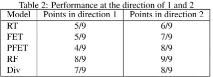
Table 2: Performance at the direction of 1 and 2 Model Points in direction 1 Points in direction 2
RT 5/9 6/9
FET 5/9 7/9
PFET 4/9 8/9
RF 8/9 9/9
Div 7/9 8/9
Table 2 and 3 show the local correction performance along dif-ferent directions and distances to the distortion center. We can see the ratio of RF model is the largest, while the FET, PFET, division model are almost the same and the RT model is the least. This result is consistent with the overall performance of the cor-responding model.
6. CONCLUSION AND RECOMMENDATIONS
Fisheye lens is widely used in such fields as robot navigation, target detection and so on. Fisheye lens calibration is the first step of image processing. This paper focuses on the evaluation of the calibration performance. Based on the observation that lines become straight after the correction of the distorted image, the Hough-based measure is proposed in this paper to evaluate the calibration performance of different distortion models.
After lots of experimental tests, the proposed evaluation measure works well. For the five calibration models, it is concluded that 1) RT model works the worst; 2) the FET model, PFET model and division model have the similar performance and work better than RT model; 3) RF model works the best in fisheye lens cor-rection in terms of precision. It is consistent with Carlos Ricolfe-Viala’s (Ricolfe-Viala and S´anchez-Salmer´on, 2010b) result and proves that the proposed evaluation measure is simple and effec-tive. As far as ease-using are concerned, the division model with one parameter can get distortion parameter automatically and on-ly needs one image with lines. It is very convenient and fast. So, in the case of non-restricted calibration, the division model is of practical use.
ACKNOWLEDGEMENTS
Map-ping (Program NO 2015AA124001), State Key Technology Re-search and Development Program (863), China.
REFERENCES
Alem´an-Flores, M., Alvarez, L., Gomez, L. and Santana-Cedr´es, D., 2014. Automatic lens distortion correction using one-parameter division models. Image Processing On Line 4, p-p. 327–343.
Arfaoui, A. and Thibault, S., 2013. Fisheye lens calibration using virtual grid. Applied optics 52(12), pp. 2577–2583.
Basu, A. and Licardie, S., 1995. Alternative models for fish-eye lenses. Pattern Recognition Letters 16(4), pp. 433–441.
Claus, D. and Fitzgibbon, A. W., 2005. A rational function lens distortion model for general cameras. In: Computer Vision and Pattern Recognition, 2005. CVPR 2005. IEEE Computer Society Conference on, Vol. 1, IEEE, pp. 213–219.
Devernay, F. and Faugeras, O., 2001. Straight lines have to be straight. Machine vision and applications 13(1), pp. 14–24.
Duane, C. B., 1971. Close-range camera calibration. Photogram-metric engineering 37(8), pp. 855–866.
Fitzgibbon, A. W., 2001. Simultaneous linear estimation of mul-tiple view geometry and lens distortion. In: Computer Vision and Pattern Recognition, 2001. CVPR 2001. Proceedings of the 2001 IEEE Computer Society Conference on, Vol. 1, IEEE, pp. I–125.
Grossberg, M. D. and Nayar, S. K., 2001. A general imaging model and a method for finding its parameters. In: Computer Vi-sion, 2001. ICCV 2001. Proceedings. Eighth IEEE International Conference on, Vol. 2, IEEE, pp. 108–115.
Hughes, C., Denny, P., Glavin, M. and Jones, E., 2010. Equidis-tant fish-eye calibration and rectification by vanishing point ex-traction. Pattern Analysis and Machine Intelligence, IEEE Trans-actions on 32(12), pp. 2289–2296.
Lee, T.-Y., Chang, T.-S., Lai, S.-H., Liu, K.-C. and Wu, H.-S., 2011. Wide-angle distortion correction by hough transform and gradient estimation. In: Visual Communications and Image Pro-cessing (VCIP), 2011 IEEE, IEEE, pp. 1–4.
Ricolfe-Viala, C. and Sanchez-Salmeron, A.-J., 2010a. Lens dis-tortion models evaluation. Appl. Opt. 49(30), pp. 5914–5928.
Ricolfe-Viala, C. and S´anchez-Salmer´on, A.-J., 2010b. Robust metric calibration of non-linear camera lens distortion. Pattern Recognition 43(4), pp. 1688–1699.
Weng, J., Cohen, P. and Herniou, M., 1992. Camera calibration with distortion models and accuracy evaluation. IEEE Transac-tions on Pattern Analysis and Machine Intelligence 14(10), p-p. 965–980.
Zhang, Y., 2012. Fisheye distorted image calibration using parabolic perspective projection constraint. In: Image and Signal Processing (CISP), 2012 5th International Congress on, IEEE, p-p. 369–372.
Zhang, Z., 2000. A flexible new technique for camera calibration. Pattern Analysis and Machine Intelligence, IEEE Transactions on 22(11), pp. 1330–1334.
(a) (b) (c)
(d) (e)
Figure 5: Results of lens correction using the RT model (a) , FET model (b), PFET model (c), RF model (d), division model (e)
(a) (b) (c)
(d) (e)
(a) (b) (c)
(d) (e)
Figure 7: The corrected corner points at the vertical direction using the RT model (a),FET model (b),PFET model (c),RF model (d),division model (e)
(a) (b) (c)
(d) (e)