ASSESSING THE UTILITY OF UAV-BORNE HYPERSPECTRAL IMAGE AND
PHOTOGRAMMETRY DERIVED 3D DATA FOR WETLAND SPECIES DISTRIBUTION
QUICK MAPPING
Q. S. Li a *, F. K.K. Wong a, T. Fung a
a Department of Geography and Resource Management, The Chinese University of Hong Kong, HKSAR –
[email protected], [email protected], [email protected]
Commission VI, WG VI/4
KEY WORDS: DSM, Feature Reduction, Hyperspectral, Photogrammetric Point Cloud, Species Mapping, UAV
ABSTRACT:
Lightweight unmanned aerial vehicle (UAV) loaded with novel sensors offers a low cost and minimum risk solution for data acquisition in complex environment. This study assessed the performance of UAV-based hyperspectral image and digital surface model (DSM) derived from photogrammetric point clouds for 13 species classification in wetland area of Hong Kong. Multiple feature reduction methods and different classifiers were compared. The best result was obtained when transformed components from minimum noise fraction (MNF) and DSM were combined in support vector machine (SVM) classifier. Wavelength regions at chlorophyll absorption green peak, red, red edge and Oxygen absorption at near infrared were identified for better species discrimination. In addition, input of DSM data reduces overestimation of low plant species and misclassification due to the shadow effect and inter-species morphological variation. This study establishes a framework for quick survey and update on wetland environment using UAV system. The findings indicate that the utility of UAV-borne hyperspectral and derived tree height information provides a solid foundation for further researches such as biological invasion monitoring and bio-parameters modelling in wetland.
* Corresponding author
1. INTRODUCTION
An accurate species distribution survey is required for effective coastal wetland ecosystem management and preservation. To this end, satellite and airborne remote sensing data has been widely used for wetland species classification (Dronova, 2015; Fabian Ewald Fassnacht et al., 2016). Hyperspectral sensors provides narrow-band and contiguous spectral data, which allows better examination and discrimination of vegetation types (Adam, Mutanga, & Rugege, 2010). Many attempts have been successfully made to classify wetland species or monitoring invasive species by high resolution hyperspectral data (Hestir et al., 2008; Kamal & Phinn, 2011; Papeş, Tupayachi, Martínez, Peterson, & Powell, 2010). Meanwhile, tree height information derived from LiDAR data was combined with hyperspectral image to improve the species classification (Ghosh, Fassnacht, Joshi, & Koch, 2014). However, limited by spatial and spectral resolution of satellite image and the high cost of manned airborne data acquisition, detail survey and monitoring of complex wetland environment is sometimes prohibited. In recent years, lightweight unmanned aerial vehicle (UAV) loading with novel sensors offers a low cost and flexible approach for data acquisition. UAV with flexible sensors is able to collect high-resolution, hyperspectral and multi-angle images for 3D terrain reconstruction. Successful researches have been conducted by utilizing UAV-borne images for tree species mapping, structure or biophysical parameter estimation and individual tree detection in forestry area (Berni, Zarco-Tejada, Suárez, & Fereres, 2009; Hill et al., 2016; Huang et al., 2016; Nevalainen et al., 2017).
Due to inter-band correlation in hyperspectral data, feature selection or extraction are usually performed to reduce data dimension and noise to improve classification efficiency. Feature selection methods select a subset from the original bands. Common selection methods include stepwise discriminate analysis, hierarchical clustering, support vector machine (SVM), partial least square discriminate analysis (PLSDA) and genetic algorithms (Fabian E. Fassnacht et al., 2014; Fung, Fung, Ma, & Siu, 1997; Pal & Foody, 2010). Feature extraction methods reduce the number of band data through data transformation with the aim to extract maximal information from the original data. Minimum noise fraction (MNF) transformation and principal component analysis (PCA) are widely applied in hyperspectral image (Burai, Deák, Valkó, & Tomor, 2015; Marcinkowska-Ochtyra et al., 2017). MNF is reported yielding higher accuracy than feature selection result or full band used result (Fabian E. Fassnacht et al., 2014).
In terms of classification, probability-based Maximum Likelihood Classifier (MLC) is a widely used traditional supervised classification algorithm that offers reasonable classification accuracy (Binaghi, Gallo, Boschetti, & Brivio, 2005; Burai et al., 2015). Machine-learning classifiers such as decision tree, artificial neural network and support vector machine (SVM) are becoming popular due to their relatively accurate and robust performance in classification exercise (Dalponte, Orka, Gobakken, Gianelle, & Naesset, 2013; Wong & Fung, 2014). SVM is a commonly used classifier for hyperspectral image. SVM separates the classes with a decision surface that maximizes the margin between the classes. SVM was reported to outperform when cope with high dimension,
limited samples and multi-source data representing complex environments (Jones, Coops, & Sharma, 2010).
The aim of study is to assess the utility of UAV-borne hyperspectral image and photogrammetry derived 3D data for detail wetland species mapping. The following aspects are considered and analysed: 1) to identify spectral regions for effective wetland species classification, 2) to examine the effect of photogrammetry-derived height data in mapping dense and complex wetland species, 3) to evaluate various classifiers for important inter-tidal habitats. There are six main habitats in Mai Po Nature Reserve: gei wais (shrimp ponds), freshwater ponds, inter-tidal mudflats, mangroves, reedbeds and fishponds (WWF). The test site is part of gei wais area, a semi-natural wetland landscape with various wetland species. In recent years, gei wai areas suffer from species invasion, which is challenging for native wetland species monitoring and preservation.
2.2 Flight Campaign and Fieldwork
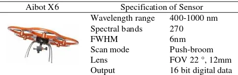
Two flight campaigns were conducted in sunny and windless weather covering an area of approximately 20000m2. An autonomously flying hexacopter Aibot X6 equipped with a pushbroom Headwall Nano-Hyperspec sensor was used to acquire a 270-band image. The UAV and specifications of hyerspectral sensor are shown in the Table 1.
Aibot X6 Specification of Sensor Wavelength range 400-1000 nm Spectral bands 270
FWHM 6nm
Scan mode Push-broom
Lens FOV 22 °, 12mm
Output 16 bit digital data Table 1. Aibot X6 and specification of hyperspectral sensor
The first flight campaign was conducted in 8th December, 2016 using Aibot X6 to collect hyperspectral images. The flight altitude was 100 meters above ground with an equivalent spatial resolution of 0.06 meter.
The second flight campaign together with species distribution survey were carried out in 29th March 2017. Normal RGB images were acquired using a DJI Phantom 4 quadcopter from five angles to the same site. The end-lap and side-lap were both set to 75%. The quadcopter flied at 50 meters above ground and the spatial resolution is 0.02 meter. Ground truth survey was implemented by combining field investigation to UAV-borne RBG image visual interpretation due to limited accessibility in the site. Major species included reed bed and three types of mangrove: Kandelia obovata, Aegiceras corniculatum and Acrostichum aureum. Other species include a pioneer mangrove: Acanthus ilicifolius, various graminaceous plants, three arbor species, one shrub species and one invasive species. In particular, invasive species Mikania micrantha climbed up to
the mangrove canopy causing morphology change to mangrove (AFCD. 2006), which might hinder effective mapping of mangrove species.
2.3 UAV Data Processing
2.3.1 Hyperspectral Data: SpectralView software (Headwall Photonics Inc., MA, U.S.) was used for radiative and geometric correction. Radiative correction was processed with the radio calibration file, which recorded the corresponding exposure time and dark current reference. The file was used to create radiance cube from raw data. The first eight bands were removed due to severe information loss and noise. Ortho-rectification was then conducted using information generated from inertial motion sensor that communicated with the Nano-hyperspec sensor during the scanning process. GPS and frame index records were used to adjust orientation while IMU/GPS offsets were used for image correction and orientation. In addition, the altitude of the scan and DEM were input to adjust the geometric distortion. UTM Zone 50 projection was applied to the hyperspectral data.
2.3.2 3D Data Generation: Generally, canopy height is estimated by subtracting digital terrain model from digital surface model (DSM). As the test site was part of shallow bay with flat terrain, variation of canopy height can be well represented by the DSM. The Agisoft PhotoScan Professional commercial software (AgiSoft LLC, St. Petersburg, Russia), was used for multi-view RGB data mosaic and point cloud generation. A total of 1,340 RGB images were loaded in Agisoft PhotoScan. After defining the camera position and orientation, images were automatically stitched together and highly dense point clouds and mesh were generated (3D polygonal model). As for the reconstruction parameter, ultra high quality was set to process original images and a mild depth filtering mode was used to automatically remove points with large uncertainty errors. An ortho-mosaic image was generated for map registration. Dense point clouds were loaded into ENVI LiDAR (Exelis Visual Information Solutions, Inc, U.S.). A 5-cm grid resolution DSM was generated in order to retain detail spatial feature. A number of ground control points were selected to apply to map registration among hyperspectral image, orthomosaic RBG image and the DSM layer.
2.4 Sample Data Selection
Based on the knowledge of fieldwork and visual interpretation, 16 classes involving 13 species, and 2 other land covers were identified. Invasive species Mikania micrantha in normal and dry growth morphology was classified as two classes. Representative training samples were manually selected. Validating samples was approximately half of training samples. 150 points were randomly extracted from training samples in each class as feature reduction test samples. Classes and sample number are shown in the appendix.
2.5 Feature Reduction
Multiple feature reduction methods were compared in this study. They include traditional statistic approach stepwise discriminant analysis (SDA), machine learning algorithm support vector machine (SVM) and data extraction method minimum noise fraction (MNF) transformation. The objective is to identify the high performance method for species classification and to explore spectral bands for better species discrimination.
Stepwise discriminant analysis (SDA) is a common statistic method to automatically select the best spectral band based on F value. Image bands would be selected by the model if the F value large than 3.84 and they would be removed if F value less than 2.71 (Fung et al., 1997). Subsequently, the predictive importance of each band was calculated to indicate the relative importance of each band in estimating the model. Support vector machine (SVM) is a robust classification and regression technique by mapping data to a high-dimensional feature space so that data points can be categorized in maximum predictive accuracy without overfitting the training data (Chang & Lin, 2001). In this experiment, a radial basis function (RBF) kernel was applied. Several SVM operations were run with slight tuning of input parameters RBF gamma and stopping criteria. Predictor importance was calculated to determine significant bands for species classification. Both feature selection methods were implemented in SPSS Modeler software (IBM Corporation, New York, U.S.).
Minimum noise fraction (MNF) transformation resembles principal component analysis to remove noise and determine the inherent dimension. It uses principal components derived from the original image data after they were noise-whitened by the first principal components rotation and were then rescaled by the noise standard deviation (Green et al.,1988). MNF transformation was implemented in the ENVI 5.1 software. Noise statistics was estimated in full hyperspectral bands. A vegetation mask was created from normalized difference vegetation index (NDVI). NDVI was calculated using ρNIR = 800nm, ρRed = 679nm (Yu, Qiu, Wang, Sun, & Wang, 2016) and threshold between 0.16 and 1.00 was considered as vegetation area through visual interpretation. In MNF transformation, non-vegetated area masked out so that the first few MNF components extracted the spectral variances from vegetation species (Fabian E. Fassnacht et al., 2014).
2.6 Classification
Two supervised classification algorithms MLC and SVM with radial basis function (RBF) kernel were tested. To be comparable, each classification algorithm used the same set of training and validating samples. The classification process was conducted in ENVI 5.1 and the default parameters of classifier in the software were used. Previous studies (Fabian E. Fassnacht et al., 2014; Fung et al., 1997; Raczko & Zagajewski, 2017) suggested that about 15-20 input bands produced the best classification result. Spectral subsets comprising the first 15-20 most importance bands extracted from SDA, SVM and MNF feature selection and extraction results were served as input. DSM was also input into classifier as auxiliary data. In addition to subset bands, all 265 bands were also input into the SVM classifier as a base for comparison. As MLC requires the number of training sample for each class to be larger than the number of input band, the all band option is not available. Using the validating samples, classification accuracy and
reliability were evaluated by confusion matrix and Kappa coefficient respectively.
3. RESULT 3.1 Spectral Region of Selected Bands
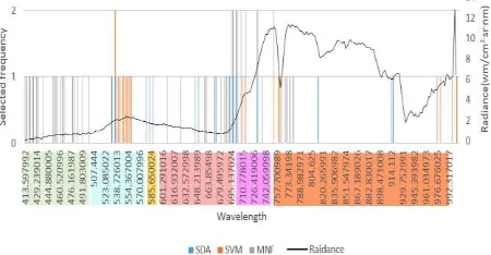
Considering the predictor importance scores of SDA, SVM and eigenvalue plot of MNF transformation, the first 20 most important bands were selected and extracted for subsequent processing. Band contribution to the first 20 MNF components was calculated by ENVI 5.1 and contribution weight large than 0.5 was regarded as important band in MNF transformation. Figure 1 shows the important band positions and selected frequency by the three data reduction methods. As shown in the frequency bar chart, selected bands frequently laid along the green peak (530-550nm), red (650-700nm), red edge (700-730nm) and oxygen absorption near infrared region (760-780nm). Compared to SVM, SDA selected chlorophyll absorption red band (650-700nm) and yellow band (570-590nm). The MNF components showed quite a different result. The first several green bands (410-490nm) contributed most instead of green peak (530-550nm). Other significant bands include red band, red edge band and near infrared oxygen absorption bands around 760-780nm, which were similar to the results from the other two band selection methods.
Figure 1. Important band position and selected frequency by three data reduction methods
3.2 Classification Results
3.2.1 Feature Reduction Methods: Extracted subsets of three feature reduction methods were input into the classifiers and the results were compared. Table 2 summarized the overall classification accuracy of different subsets. As this main objective of this study is to assess UAV-borne data for species mapping, only vegetation classes were included to calculate the overall accuracy. Classification results of both classifiers showed that subsets of MNF transformation performed the best (MLC: 88.91%; SVM: 88.02%), followed by SDA (MLC: 76.95%; SVM: 73.74%) and SVM with RBF kernel and gamma value at 0.1 performed the worst (MLC: 64.41%; SVM: 65.07%). MNF transformation accuracy was even better than the results using all bands.
Input bands/Classifier MLC SVM
OA Kappa OA Kappa
SDA 20 bands 76.95% 0.748 73.74% 0.712
SVM 20 bands 64.41% 0.611 65.07% 0.616
MNF 20 components 88.91% 0.880 88.02% 0.868
All 265 bands 79.84% 0.779
SDA 20 bands + DSM 81.20% 0.794 77.97% 0.758
MNF 20 components + DSM
89.07% 0.880 89.07% 0.880
Table 2. Overall classification accuracy of different subsets (OA: overall accuracy)
3.2.2 Auxiliary DSM Data: Since MNF and SDA subsets obtained acceptable classification accuracy, DSM data was added in these two spectral subsets for subsequent comparison. As shown in Table 2, overall accuracy and Kappa coefficient have been improved after adding DSM data. Figure 2 compares the overall classification accuracy and producer’s accuracy of each species with and without input of DSM data to MNF and SDA subset in SVM classifier. Generally, the DSM data improves overall accuracy and producer’s accuracy and this improvement was more obvious when combining with SDA subset than MNF subset. For SDA subset, the overall accuracy enhanced from 76.95% to 81.20% and from 73.74% to 77.97% for MLC and SVM classifiers respectively. For MNF subset, the enhancement is not as significant as that of SDA with less than 1% increase in overall accuracy. Among all of the classification runs, subset of MNF 20 components and DSM yielded the best classification accuracy.
Figure 2. Overall and producer’s accuracy of before and after adding DSM data by SVM Classifier
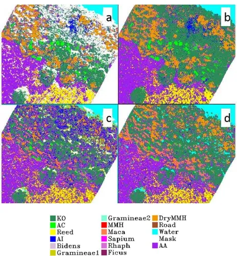
Besides, visual interpretation of classification maps showed in Figure 3 indicated that DSM data enhanced the discriminant capacity among low plants such as Acanthus ilicifolius and Acrostichum aureum, arbor and mangrove species Kandelia obovata. Meanwhile, DSM reduced misclassification due to the shadow effect and morphological variation of mangrove Kandelia obovata.
Figure 3. SVM classification map before and after adding DSM data (a: MNF 20 components; b: MNF 20 components + DSM;
c: SDA 20 bands; d: SDA 20 bands + DSM)
3.2.3 Classifiers: As shown in the Table 2, both classifier obtained approximate overall accuracy and Kappa coefficient with the same input subset. While MLC obtained a slightly higher overall accuracy than SVM Classifier when using the MNF components (MLC: 88.91%, SVM: 88.02%) and SDA selected bands (MLC: 76.95%, SVM: 73.74%).
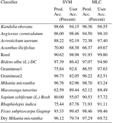
Apart from quantitative accuracy assessment, visual interpretation of classification maps was also carried out. Figure 4 shows the areal proportion of each class based on the output from compared classifier. Although both classifiers showed an overestimation in less common species such as non-mangrove arbor and Gramineae, SVM classifier gave better classification result than MLC as shown in Figure 5. Specifically, in terms of mangrove species, MLC overestimated the Acanthus ilicifolius and underestimated Kandelia obovata. The adjacent boundary between mangrove and water were misclassified to reed and dry Mikania micrantha. Similar misclassification occurred in MNF and SDA band subsets. Moreover, map comparison results indicated that SVM classifier reduced scattered patches and eliminated salt-and-pepper effect that were noticeable in MLC result. Last but not the least, SVM classifier made better use of DSM data than MLC when identified different mangrove species as misclassification due to shadow effect and morphological variation of inter-species were reduced effectively in SVM classification result. As shown in the Table 3, SVM classifier yielded higher producer accuracy than MLC in four mangrove species Kandelia obovata, Aegiceras corniculatum, Acrostichum aureum and Acanthus ilicifolius.
Based on the above analysis, SVM classifier was more preferable than MLC when combining hyperspectral and DSM data for species mapping.
Figure 4. Areal proportion of 16 classes based on classification result
Figure 5. Classification map of MNF 20 components + DSM (a: SVM classifier; b: MLC)
Classifier SVM MLC
Prod. Acc.
User Acc.
Prod. Acc.
User Acc. (Percent) (Percent)
Kandelia obovata 98.66 94.15 96.36 96.55
Aegiceras corniculatum 96.00 98.46 94.50 98.10
Acrostichum aureum 88.22 92.19 72.38 97.40
Acanthus ilicifolius 70.80 68.38 66.37 49.67
Reed 90.62 98.98 91.93 99.80
Bidens alba (L.) DC 97.39 86.42 97.07 94.90
Gramineae1 75.84 92.8 86.55 97.63
Gramineae2 96.73 82.05 96.22 82.51
Mikania micrantha 96.76 82.96 98.70 83.24
Macaranga tanarius 62.59 89.44 62.12 88.49
Sapium sebiferum (L.) Roxb 80.00 55.07 90.53 57.72
Rhaphiolepis indica 75.44 87.76 71.93 91.11
Ficus subpisocarpa Gagnep 93.33 99.45 98.46 98.46
Dry Mikania micrantha 96.12 79.74 97.29 69.72
Table 3. Producer and user accuracy for each class using MNF 20 components and DSM as input
4. DISCUSSION 4.1 Feature Reduction Methods
Results from feature reduction analyses suggested that four spectral regions were important for wetland species discrimination. Consistent with previous researches (Clark et al., 2005; Fabian E. Fassnacht et al., 2014; Fung et al., 1997), spectral wavelengths at 520-620nm and 690-770nm included the chlorophyll absorption green peak, red, red edge and O2 absorption region, which are related to pigment contents and cell structure were useful in species classification.
In terms of feature reduction methods, SVM selected bands clustered around green peak, red edge and NIR region but omitted information from other spectral regions. In contrast, bands selected by SDA indicated other significant regions such as O2 absorption regions around 760nm and NIR around 900nm. Additionally, SDA selected yellow bands to help distinguish withered plants like reed and Dry invasive Mikania micrantha. Therefore, SDA subset was able to obtain better accuracy than SVM subset. Particularly, bands at 410-490nm contribute significantly to MNF components, which suggested significance of green bands in species classification.
Same as the result from (Fabian E. Fassnacht et al., 2014), feature selected methods are not comparable with MNF feature extraction methods. MNF transformation produced the best classification map and accuracy by removing noise and retaining the most of the significant spectral feature at the same time. One drawback of MNF method was that the transformation components were unable to represent the physical objects. Although band contribution in each component can be analyzed, it was still hard to study the species distinguishing mechanism in view of the selected components. More sophisicated feature selection methods such as partial least square discriminant analysis (PLSDA) (Fabian E. Fassnacht et al., 2014) and improved SVM (Pal & Foody, 2010) should be used to identify the significant and robust spectrum for species classification and bio-parameters modelling in future work.
4.2 3D Data Digital Surface Model (DSM)
There were two obvious and significant improvement after adding DSM data to classifier. Firstly, DSM largely reduced misclassification due to the shadow effect and morphological variation of inter-species in the study area. In some areas, invasive species such as Mikania micrantha covered the mangrove canopy, which made mangrove sparse or even die. On one hand, the diseased mangroves cause morphological change, which resulted in larger variation of spectral reflectance. For instance, Kandelia obovata suffered invasion appears more sparse and darker than healthy Kandelia obovata. On the other hand, the spreading vines of invasive species covering the mangrove canopy results in mixed pixels. Therefore, most of the invaded areas were unclassified or misclassified as low radiance species such as Acrostichum aureum. With DSM added, the height information somehow offset these impacts and assigned diseased mangrove pixels to correct class. Secondly, canopy height information was especially useful in distinguishing species with large height difference such as Kandelia obovata, and Acrostichum aureum and thus reduced the overestimation of low species such as Acanthus ilicifolius and Acrostichum aureum.
4.3 Classifier
The visual interpretation and accuracy assessment result indicated that SVM classifier is more applicable than MLC when hyperspectral subset and terrain data were combined. SVM classifier produced more reasonable classification map although it did not obtain the highest classification accuracy in most of the classification runs. Previous researches also suggested that SVM classifier outperformed conventional approaches to classify high-dimensional and multi-source data in complex environments (Jones, Coops, & Sharma, 2010). Due to non-linear and adaptive fitting capacities of RBF kernel, SVM was powerful to cope with high dimension data (Verrelst et al., 2015). However, the drawback of SVM classifier was the relatively long execution time in the model building process. Other factors that affected the classification accuracy and stability such as pixel number of training sample, parameters tuning of classifier etc. should be explored in future study.
5. CONCLUSION
This study established a framework of using UAV system for quick mapping of 13 species in a mixed and complex wetland environment with desirable classification accuracy. With the assistance of UAV system, it offered a solution for detail species survey of wetland area in relatively low cost of time and labour. Significant spectral regions were identified, effect of terrain data were assessed and classifiers were evaluated. The findings suggested that the utility of UAV-borne hyperspectral and photogrammetry-derived 3D data help to characterize and monitor wetland environment, which provide basic information for further researches such as biological invasion monitoring and bio-parameters modelling.
ACKNOWLEDGEMENTS
This paper is part of the research work carried out in the project U516187 financed by General Research Fund Grant, Research Grants Council (RGC) of Hong Kong.
REFERENCES
Adam, E., Mutanga, O., & Rugege, D. (2010). Multispectral and hyperspectral remote sensing for identification and mapping of wetland vegetation: A review. Wetlands Ecology and Management, 18(3), pp. 281–296.
Berni, J., Zarco-Tejada, P. J., Suárez, L., & Fereres, E. (2009). Thermal and narrowband multispectral remote sensing for vegetation monitoring from an unmanned aerial vehicle. Geoscience and Remote Sensing, {IEEE} Transactions on, 47(3), pp. 722–738.
Binaghi, E., Gallo, I., Boschetti, M., & Brivio, P. A. (2005). A Neural Adaptive Algorithm for Feature Selection and Classification of High Dimensionality Data (pp. 753–760). Springer, Berlin, Heidelberg.
Burai, P., Deák, B., Valkó, O., & Tomor, T. (2015). Classification of Herbaceous Vegetation Using Airborne Hyperspectral Imagery. Remote Sensing, 7(2), pp. 2046–2066.
Clark, M. L., Roberts, D. A., & Clark, D. B. (2005). Hyperspectral discrimination of tropical rain forest tree species
at leaf to crown scales. Remote Sensing of Environment, 96(3), pp. 375–398.
Dalponte, M., Orka, H. O., Gobakken, T., Gianelle, D., & Naesset, E. (2013). Tree Species Classification in Boreal Forests With Hyperspectral Data. IEEE Transactions on Geoscience and Remote Sensing, 51(5), pp. 2632–2645.
Dronova, I. (2015). Object-based image analysis in wetland research: A review. Remote Sensing, 7(5), pp. 6380–6413.
Fassnacht, F. E., Latifi, H., Stereńczak, K., Modzelewska, A., Lefsky, M., Waser, L. T., Ghosh, A. (2016). Review of studies on tree species classification from remotely sensed data. Remote Sensing of Environment, 186, pp. 64–87.
Fassnacht, F. E., Neumann, C., Forster, M., Buddenbaum, H., Ghosh, A., Clasen, A., Koch, B. (2014). Comparison of Feature Reduction Algorithms for Classifying Tree Species With Hyperspectral Data on Three Central European Test Sites. IEEE Journal of Selected Topics in Applied Earth Observations and Remote Sensing, 7(6), pp. 2547–2561.
Fung, T., Fung, H., Ma, Y., & Siu, W. L. (1997). Band Selection Using Hyperspectral Data of Subtropical Tree Species. Geocarto International.
Ghosh, A., Fassnacht, F. E., Joshi, P. K., & Koch, B. (2014). A framework for mapping tree species combining hyperspectral and LiDAR data: Role of selected classifiers and sensor across three spatial scales. International Journal of Applied Earth Observation and Geoinformation, 26, pp. 49–63.
Hestir, E. L., Khanna, S., Andrew, M. E., Santos, M. J., Viers, J. H., Greenberg, J. A., Ustin, S. L. (2008). Identification of invasive vegetation using hyperspectral remote sensing in the California Delta ecosystem. Remote Sensing of Environment, 112(11), pp. 4034–4047.
Hill, D. J., Tarasoff, C., Whitworth, G. E., Baron, J., Bradshaw, J. L., & Church, J. S. (2016). Utility of unmanned aerial vehicles for mapping invasive plant species: a case study on yellow flag iris ( Iris pseudacorus L.). International Journal of Remote Sensing, pp. 1–23.
Huang, J., Sun, Y., Wang, M., Zhang, D., Sada, R., & Li, M. (2016). Juvenile tree classification based on hyperspectral image acquired from an unmanned aerial vehicle. International Journal of Remote Sensing, pp. 1–23.
Jones, T. G., Coops, N. C., & Sharma, T. (2010). Assessing the utility of airborne hyperspectral and LiDAR data for species distribution mapping in the coastal Pacific Northwest, Canada. Remote Sensing of Environment, 114(12), pp. 2841–2852.
Kamal, M., & Phinn, S. (2011). Hyperspectral data for mangrove species mapping: A comparison of pixel-based and object-based approach. Remote Sensing, 3(10), pp. 2222–2242.
Marcinkowska-Ochtyra, A., Zagajewski, B., Ochtyra, A., Jarocińska, A., Wojtuń, B., Rogass, C., … Lavender, S. (2017). Subalpine and alpine vegetation classification based on hyperspectral APEX and simulated EnMAP images. International Journal of Remote Sensing, pp. 1–26.
Nevalainen, O., Honkavaara, E., Tuominen, S., Viljanen, N., Hakala, T., Yu, X., … Tommaselli, A. (2017). Individual Tree
Detection and Classification with UAV-Based Photogrammetric Point Clouds and Hyperspectral Imaging. Remote Sensing, 9(3), pp. 185.
Pal, M., & Foody, G. M. (2010). Feature Selection for Classification of Hyperspectral Data by SVM. IEEE Transactions on Geoscience and Remote Sensing, 48(5), pp. 2297–2307.
Papeş, M., Tupayachi, R., Martínez, P., Peterson, A. T., & Powell, G. V. N. (2010). Using hyperspectral satellite imagery for regional inventories: a test with tropical emergent trees in the Amazon Basin. Journal of Vegetation Science, 21(2), pp. 342–354.
Raczko, E., & Zagajewski, B. (2017). Comparison of support vector machine, random forest and neural network classifiers for tree species classification on airborne hyperspectral APEX images. European Journal of Remote Sensing, 50(1), pp. 144– 154.
Verrelst, J., Camps-Valls, G., Muñoz-Marí, J., Rivera, J. P., Veroustraete, F., Clevers, J. G. P. W., & Moreno, J. (2015). Optical remote sensing and the retrieval of terrestrial vegetation bio-geophysical properties – A review. ISPRS Journal of Photogrammetry and Remote Sensing, 108, pp. 273–290.
Wong, F. K. K., & Fung, T. (2014). Combining EO-1 Hyperion and Envisat ASAR data for mangrove species classification in Mai Po Ramsar Site, Hong Kong. International Journal of Remote Sensing, 35(23), pp. 7828–7856.
Yu, K., Qiu, L., Wang, J., Sun, L., & Wang, Z. (2016). Winter wheat straw return monitoring by UAVs observations at different resolutions. International Journal of Remote Sensing, pp. 1–13.
APPENDIX Summary of sample data Classes Training
samples (Pixel)
Validating samples (Pixel)
Test samples for feature reduction (Pixel) Kandelia
obovata
1102 552 150
Aegiceras corniculatum
997 600 150
Reed 1005 533 150
Acrostichum aureum
1014 362 150
Acanthus ilicifolius
258 113 150
Bidens alba (L.) DC
711 307 150
Gramineae1 1078 476 150
Gramineae2 1106 397 150
Mikania micrantha
1016 463 150
Macaranga tanarius
985 433 150
Sapium sebiferum (L.) Roxb
283 95 150
Rhaphiolepis indica
158 57 150
Ficus subpisocarpa Gagnep
330 195 150
Dry Mikania
micrantha
696 258 150
Road 616 317 150
Water 1016 497 150