Agriculture, Ecosystems and Environment 82 (2000) 139–158
Consequences of future climate change and changing climate
variability on maize yields in the midwestern United States
Jane Southworth
a,∗, J.C. Randolph
a, M. Habeck
b, O.C. Doering
b,
R.A. Pfeifer
b, D.G. Rao
c, J.J. Johnston
aaSchool of Public and Environmental Affairs, Indiana University, 1315 E. Tenth Street, Bloomington, IN 47405-1701, USA bDepartment of Agricultural Economics, Purdue University, West Lafayette, IN, USA
cCentral Research Institute for Dryland Agriculture, Hyderabad, India
Abstract
Any change in climate will have implications for climate-sensitive systems such as agriculture, forestry, and some other natural resources. With respect to agriculture, changes in solar radiation, temperature, and precipitation will produce changes in crop yields, crop mix, cropping systems, scheduling of field operations, grain moisture content at harvest, and hence, on the economics of agriculture including changes in farm profitability. Such issues are addressed for 10 representative agricultural areas across the midwestern Great Lakes region, a five-state area including Indiana, Illinois, Ohio, Michigan, and Wisconsin. This region is one of the most productive and important agricultural regions in the world, with over 61% of the land use devoted to agriculture.
Individual crop growth processes are affected differently by climate change. A seasonal rise in temperature will increase the developmental rate of the crop, resulting in an earlier harvest. Heat stress may result in negative effects on crop production. Conversely, increased rainfall in drier areas may allow the photosynthetic rate of the crop to increase, resulting in higher yields. Properly validated crop simulation models can be used to combine the environmental effects on crop physiological processes and to evaluate the consequences of such influences. With existing hybrids, an overall pattern of decreasing crop production under scenarios of climate change was found, due primarily to intense heat during the main growth period. However, the results changed with the hybrid of maize (Zea mays L.) being grown and the specific location in the study region. In general, crops grown in sites in northern states had increased yields under climate change, with those grown in sites in the southern states of the region having decreased yields under climate change. Yields from long-season maize increased significantly in the northern part of the study region under future climate change. Across the study region, long-season maize performed most successfully under future climate scenarios compared to current yields, followed by medium-season and then short-season varieties. This analysis highlights the spatial variability of crop responses to changed environmental conditions. In addition, scenarios of increased climate variability produced diverse yields on a year-to-year basis and had increased risk of a low yield. Results indicate that potential future adaptations to climate change for maize yields would require either increased tolerance of maximum summer temperatures in existing maize varieties or a change in the maize varieties grown. © 2000 Elsevier Science B.V. All rights reserved.
Keywords: Climate change; Variability; CERES-maize; Maize yields; Agriculture; Midwestern United States
∗Corresponding author. Tel:+1-812-855-4953; fax:+1-812-855-7547.
E-mail address: [email protected] (J. Southworth).
1. Introduction
Interest in the consequences of increasing atmo-spheric CO2concentration and its role in influencing
climate change can be traced as far back as 1827, although more commonly attributed to the work of Arrhenius (1896) and Chamberlain (1897), as cited in Chiotti and Johnston (1995). A century later, concern over climatic change has reached global dimensions and concerted international efforts have been initiated in recent years to address this problem (Intergov-ernmental Panel on Climate Change (IPCC, 1995, 1990)). Future climate change could have significant impacts on agriculture, especially the combined ef-fects of elevated temperatures, increased probability of droughts, and a reduced crop-water availability (Chiotti and Johnston, 1995).
Based on climate records, average global tem-peratures at the earth’s surface are rising. Since global records began in the mid-19th century, the five warmest years have occurred during the 1990s and 10 of the 11 warmest years have occurred since 1980 (Pearce, 1997). Based on a range of several current climate models (IPCC, 1995, 1990), the mean annual global surface temperature is projected to increase by 1 to 3.5◦C by the year 2100 and there will be changes in the spatial and temporal patterns of precipitation (IPCC, 1995).
The variability of the climate, under current and future climate scenarios, has been a topic of recent interest for a number of reasons. The consequences of changes in variability may be as important as those that arise due to variations in mean climatic vari-ables (Hulme et al., 1999; Carnell and Senior, 1998; Semenov and Barrow, 1997; Liang et al., 1995; Rind, 1991; Mearns et al., 1984). While most studies of climate change impacts on agriculture have analyzed effects of mean changes of climatic variables on crop production, impacts of changes in climate variability have been much less studied (Mearns et al., 1997; Mearns, 1995).
Within more recent historical records, there have been significant periods of climatic fluctuations such as the dustbowl conditions of the 1930s in the United States, when the dramatic and negative effects of climate variability on agriculture were realized. Katz and Brown (1992) showed that for a given climate variable a change in the variance has a larger effect on
agricultural cropping systems than does a change in the mean. The effect of possible changes in climatic variability remains a significant uncertainty that de-serves additional attention within integrated climate change assessments (Barrow et al., 1996; Mearns et al., 1996; Semenov et al., 1996). The study of economic effects of climate change on agriculture is particularly important because agriculture is among the more climate sensitive sectors (Kane et al., 1992). Changes in climate will interact with adaptations to increase agricultural production affecting crop yields and productivity in different ways depending on the hybrids and cropping systems in a region. Important direct effects will be through changes in temperature, precipitation, length of growing season, and timing of extreme or critical threshold events relative to crop development (Saarikko and Carter, 1996). Also, an increased atmospheric CO2 concentration could have
a beneficial effect on the growth of some species. Indirect effects will include potentially detrimental changes in diseases, pests, and weeds, the effects of which have not yet been quantified in most studies. Evidence continues to support the findings of the IPCC that “global agricultural production could be main-tained relative to baseline production” for a growing population under 2×CO2 equilibrium climate
con-ditions (Rosenzweig and Hillel, 1998, 1993). In mid-dle and high latitudes, climate change will extend the length of the potential growing season, allowing earlier planting of crops in the spring, earlier maturation and harvesting, and the possibility of two or more crop-ping cycles during the same season. Climate change also will modify rainfall, evaporation, runoff, and soil moisture storage. Both changes in total seasonal pre-cipitation or in its pattern of variability are important to agriculture. Moisture stress and/or extreme heat dur-ing flowerdur-ing, pollination, and grain filldur-ing is harmful to most crops, such as maize, soybeans, and wheat (Rosenzweig and Hillel, 1993), the most important commodity crops in the midwestern United States.
J. Southworth et al. / Agriculture, Ecosystems and Environment 82 (2000) 139–158 141
Belt regions and positive effects in northern plains and western regions. More moderate warming produced estimates of predominately positive effects in some warm-season crops (IPCC, 1995).
Agricultural systems are managed and farmers always have a number of possible adaptations or op-tions open to them. These adaptation strategies may potentially lessen future yield losses from climate change or may improve yields in regions where ben-eficial climate changes occur (Kaiser et al., 1995). Thus, agricultural production responds both to phy-siological changes in crops due to climate change and also to changes in agricultural management prac-tices, crop prices, costs and availability of inputs, and government policies (Adams et al., 1999).
This research addresses the issues of changing mean climatic conditions and changes in the variabi-lity of climate around these means. The occurrence and frequency of extreme events will become increas-ingly important. This study addresses these issues for 10 representative agricultural areas in the mid-western United States for three hybrids of maize in terms of their current and future yields. Changes in climatic patterns may result in spatial shifts of agri-cultural practices, thereby impacting current land use patterns. Specifically, this research addresses (1) how the mean changes in future climate will affect maize yields across the study region for two future climate scenarios, (2) how the changes in climate variability, in addition to changes in the mean, affect poten-tial future maize yields, (3) the implications of such changes spatially, examining potential future gains and losses, and (4) some possible future adaptation strategies.
2. Methods and materials
2.1. Study region
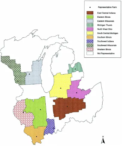
The midwestern Great Lakes region (Indiana, Illi-nois, Ohio, Michigan, and Wisconsin) was divided into 10 agricultural areas based on climate, soils, land use, and current agricultural practices. Representative farms were created in each area based upon local char-acteristics and farm endowments (Fig. 1). This region is one of the most productive and important agricul-tural regions in the world (Smith and Tirpak, 1989).
2.2. Maize crop model
The decision support system for agrotechnology transfer (DSSAT) software is a set of crop models that share a common input–output data format. The DSSAT itself is a shell that allows the user to organize and manipulate crops, soils, and weather data and to run crop models in various ways and analyze their out-puts (Thornton et al., 1997; Hoogenboom et al., 1995). The version of DSSAT used in this analysis was that supplied by ISBNAT, which is DSSAT 3.5.
Crop growth was simulated using the CERES-maize model, with a daily time step from sowing to matu-rity, based on physiological processes that describe the crop’s response to soil and aerial environmental conditions. Phasic development is quantified accord-ing to the plant’s physiological age. In CERES-maize, sub-models treat leaf area development, dry matter production, assimilate partitioning, and tiller growth and development. Potential growth is dependent on photosynthetically active radiation and its intercep-tion, whereas actual biomass production on any day is constrained by sub-optimal temperatures, soil wa-ter deficits, and nitrogen and phosphorus deficiencies. The input data required to run the CERES-maize model includes daily weather information (maximum and minimum temperatures, rainfall, and solar radia-tion); soil characterization data (data by soil layer on extractable nitrogen and phosphorous and soil water content); a set of genetic coefficients characterizing the hybrid being grown (Table 1); and crop manage-ment information, such as emerged plant population, row spacing, and seeding depth, and fertilizer and irrigation schedules (Thornton et al., 1997). The soil data were obtained from US Soil Conservation Ser-vice (SCS; now known as the Natural Resources Con-servation Service) for the 10 farm sites. The model apportions the rain received on any day into runoff and infiltration into the soil, using the runoff curve number technique. A runoff curve number was as-signed to each soil, based on the soil type, depth and texture as obtained from the STATSGO databases.
Concentrations of nitrogen and phosphorous in the soil were not limiting to crop growth and these mod-ules are turned off within the CERES-maize model runs.
J. Southworth et al. / Agriculture, Ecosystems and Environment 82 (2000) 139–158 143 Table 1
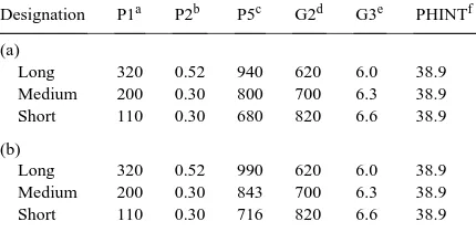
Genetic coefficients for CERES-maize for (a) east-central Indiana, south-central Michigan, eastern Wisconsin, south-west Wisconsin, and the Michigan thumb, and for (b) eastern Illinois, southern Illinois, south-west Indiana, and western Illinois
Designation P1a P2b P5c G2d G3e PHINTf (a)
Long 320 0.52 940 620 6.0 38.9 Medium 200 0.30 800 700 6.3 38.9 Short 110 0.30 680 820 6.6 38.9 (b)
Long 320 0.52 990 620 6.0 38.9 Medium 200 0.30 843 700 6.3 38.9 Short 110 0.30 716 820 6.6 38.9
aThermal time from seedling emergence to the end of the juvenile phase (expressed in degree days above a base temperature of 8◦C) during which the plant is not responsive to changes in photoperiod.
bExtent to which development (expressed as days) is delayed for each hour increase in photoperiod above the longest photope-riod at which development proceeds at a maximum rate (which is considered to be 12.5 h).
cThermal time from silking to physiological maturity (expres-sed in degree days above a base temperature of 8◦C).
dMaximum possible number of kernels per plant.
eKernel filling rate during the linear grain filling stage and under optimum conditions (mg/day).
fPhylochron interval; the interval in thermal time (degree days) between successive leaf tip appearances.
concentrations on photosynthesis and water use by the crop. Daily potential transpiration calculations are modified by the CO2 concentrations (Lal et al.,
1998; Dhakhwa et al., 1997; Phillips et al., 1996). Hence, under current conditions the model can run under the current atmospheric CO2 concentration,
approximately 360 ppmv. However, when evaluating crop growth under changed climate scenarios, which are based on the assumption of global warming due to increased concentration of CO2 (and other
green-house gases), the CO2 concentration was increased
accordingly. The atmospheric CO2 concentration for
the future climate scenarios used in this research, based on the years 2050–2059, is 555 ppmv.
CERES-maize does not have an algorithm that “kills” maize as a result of spring freezes. Hence, in this analysis, whenever a minimum air temperature of −2.0◦C or less occurred during the spring (Julian Days 1–180) and after the emergence date, growth was terminated. This value of termination was based
on discussion with Dr. Joe Ritchie (personal commu-nicatin, 1999) as being a realistic number for freeze loss of maize.
The selection of CERES-maize as the model for this research was based on (1) the daily time step of the model allows us to address the issue of changes in planting dates, (2) plant growth dependence on both mean daily temperatures and the amplitude of daily temperature values was desired (not just a daily mean temperature growth dependence as for EPIC), (3) the model simulates crop response to major climate vari-ables, including the effects of soil characteristics on water availability, and is physiologically oriented, (4) the model is developed with compatible data struc-tures so that the same soil and climate datasets can be used for all hybrids of crops which helps in com-parison (Adams et al., 1990), and (5) comprehensive validation has been done across a wide range of dif-ferent climate and soil conditions, and for difdif-ferent crop hybrids (Semenov et al., 1996; Wolf et al., 1996; Hoogenboom et al., 1995).
2.3. Crop model validation
CERES-maize has been extensively validated at sites both in the United States and abroad (Dhakhwa et al., 1997; Hoogenboom et al., 1995). Mavromatis and Jones (1998) found that using the CERES-wheat model coupled with a weather generator (WGEN or SIMMETEO) to simulate daily weather from monthly mean values is an efficient method for assessing the impacts of changing climate on agricultural produc-tion. Properly validated crop simulation models can be used to determine the influences of changes in environment, such as climate change, on crop growth (Peiris et al., 1996).
J. Southworth et al. / Agriculture, Ecosystems and Environment 82 (2000) 139–158 145
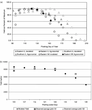
Simulated yields corresponded to within+/−10% of the observed maize yields. Overall response of simu-lated yields to planting date variation compared very favorably with observed yields.
In addition, each representative farm was validated using historical yield data and past daily climate in-formation. This validation was used to ensure the model could replicate past yields, at each location being modeled, for longer-season (currently grown) maize varieties and that the medium and short-season maize varieties showed the correct trends based on expert opinions of agronomists (Fig. 2b).
In addition, CERES-maize was used to simulate the relationships between planting date and yield (ex-pressed as a percentage of the highest yield observed for any combination of hybrid and planting date) for long, medium, and short-season maize varieties for 20 different planting dates. The relationship between planting date and yield suggest that long-season maize has higher yields than medium and short-season maize for earlier planting dates, medium-season maize has the highest yields for the middle planting dates, and short-season maize has the highest yields for late planting dates. These results are consistent with ex-pectations about hybrid performance in this region. Further, the close match between the long-season hy-brid performance and agronomist expectations gives us confidence that the model is able to describe the relationship between planting date and maize yield for these locations (Fig. 2b). Similar results have been obtained for all 10 representative agricultural areas in the study region.
2.4. Current climate analysis: VEMAP
The VEMAP dataset includes daily, monthly, and annual climate data for the conterminous United States including maximum, minimum, and mean tem-perature, precipitation, solar radiation, and humidity (Kittel et al., 1996). The VEMAP baseline (30-year historical mean) climate data was used for each of the 10 representative agricultural areas in the study region. The weather generator SIMMETEO (as used in DSSAT version 3.5) used these climate data to stochastically generate daily weather data in model runs. This approach of using monthly data to generate daily data allowed us to generate variability scenarios. The climate variables distribution patterns mimic the
current climate variables distributions. As there is no way to know future distributions, they are based on current patterns. Sensitivity analysis determined the effects of differing climatic conditions upon differing combinations of planting and harvest dates.
2.5. Future climate scenarios
This research used the Hadley Center model ‘HadCM2’ from England for future climate scenario data. This model was created from the Unified Model, which was modified slightly to produce a new, cou-pled ocean-atmosphere GCM, referred to as HadCM2. This has been used in a series of transient climate change experiments using historic and future green-house gas and sulfate aerosol forcing. These models simulate time-dependent climate change (Barrow et al., 1996). Transient model experiments are consi-dered more physically realistic and complex, and allow atmospheric concentrations of CO2to rise
grad-ually over time (Harrison and Butterfield, 1996). The results from this model have been validated at a num-ber of locations. HadCM2 is also one of the models used in the US National Assessment project.
HadCM2 has a spatial resolution of 2.5◦×3.75◦ (latitude by longitude) and the representation produces a grid box resolution of 96×73 grid cells, which pro-duces a surface spatial resolution of about 417 km× 278 km reducing to 295 km×278 km at 45◦north and south. The atmospheric component of HadCM2 has 19 levels and the ocean component 20 levels. The equili-brium sensitivity of HadCM2, that is the global-mean temperature response to a doubling of effective CO2
concentration, is 2.5◦C, somewhat lower than most other GCMs (IPCC, 1990).
The greenhouse-gas-only version, HadCM2-GHG, used the combined forcing of all the greenhouse gases as an equivalent CO2 concentration. HadCM2-SUL
used the combined equivalent CO2concentration plus
of an increase in clear-sky surface albedo proportional to the local sulfate loading (Carnell and Senior, 1998). The indirect effects of aerosols were not simulated.
Our research used the period of 2050–2059 for climate scenarios. However, using a single scenario has limitations, as it is not possible to capture the range of uncertainties as described by the IPCC. This study used two model scenarios to represent the likely upper and lower boundaries of future (2050’s) climate change. The results from HadCM2-GHG and HadCM2-SUL cannot be viewed as a forecast or prediction, but rather as two possible realizations of how the climate system may respond to a given for-cing. A comparison of the main three climate datasets (Table 2) highlights the differences in projected mean climate data for the study region. Also, a climate variability analysis was conducted on these two sce-narios, thus increasing the number of future climate scenarios to six. Hence, a range of probable climate change scenarios were examined to determine their impacts on maize growth.
2.6. Climate variability analysis
In order to separate crop response to changes in climatic means from its response to changes in climate variability, it is necessary first to model the impacts of mean temperature changes on crop growth. Then a time series of climate variables with changed variabi-lity can be constructed and added to the mean change scenarios. Hence, when the analysis is undertaken on future mean and variability changes, it is, therefore, possible to infer what type of climate change caused changes in yield (Mearns, 1995).
The mean conditions for the period 2050–2059 for each location, individual future years of climate data, and both GCM model runs were used in this analysis. The variance of the time series was changed for both temperature (maximum and minimum) and preci-pitation in time steps of one month. The variance of each month was altered separately, according to the following algorithm from Mearns (1995):
Xt0=µ+δ1/2(X
t−µ) (1)
and
δ= σ02
σ2 (2)
whereX0t is the new value of climate variable Xt (e.g. monthly mean maximum February temperature for year t),µthe mean of the time series (e.g. the mean of the monthly mean maximum February temperatures for a series of years),δthe ratio of the new to the old variance of the new and old time series, Xt the old value of climate variable (e.g. the original monthly mean February temperature for year t),σ02 the new variance, andσ2the old variance.
To change the time series to have a new variance
σ02, the variance and mean of the original time series
was calculated and then a new ratio (δ) was chosen (e.g. halving the variance). From the parametersµ,
δ, and the original time series, a new time series with variance was calculated using equation one. This al-gorithm was used to change both maximum and min-imum temperatures and the precipitation time series. This simple method, as developed by Mearns (1995) was used despite more complex methodologies be-ing developed, due to the comparisons of variability techniques. Mearns et al., (1996, 1997) illustrated the results obtained from the more computation-ally advanced, upper-level statistical techniques were surprisingly similar to prior results from the more statistically simple methodologies. If anything, these researchers noted a likelihood of underestimating the negative impacts of climate variability on crop yields using the simpler techniques, but in these analyses the differences were quite minor. The approach used here permits the incorporation of changes in both the mean and the variability of future climate in a computationally inexpensive, highly consistent, and reproducible manner.
2.7. Model and data limitations
This study does not attempt to predict future cli-mate, but rather, is an evaluation of possible future changes in agricultural production in the midwestern United States that might result from future changes in climate. Such potential changes provide insight into possible larger societal changes needed to control and reduce CO2in the atmosphere and to help select
appro-priate strategies to prepare for change (Adams et al., 1990).
J.
Southworth
et
al.
/Agricultur
e,
Ecosystems
and
En
vir
onment
82
(2000)
139–158
extreme climate-related events such as droughts or floods are not taken into account by the model in terms of extreme crop losses resulting from such events.
Other limitations relate to the simplified reality represented by the representative farms, the use of a single soil type at each location, and hence, the loss of the spatial variability of soils, although the selected soil type was that predominant at each loca-tion. However, the extensive validation and analysis at the farm level is in itself a more detailed analysis than previously undertaken.
Preparing agriculture for adaptation to climate change requires advance knowledge of how climate will change and when. The direct physical effects on plants and the indirect effects on soils, water, and other biophysical factors also must be understood. Currently, such knowledge is not available for either the direct or indirect effects of climate change. How-ever, guidance can be obtained from an improved understanding of current climatic vulnerabilities of agriculture and its resource base. This knowledge can be obtained from the use of a realistic range of climate change scenarios and from the inclusion of the com-plexity of current agricultural systems and the range of adaptation techniques and policies now available and likely to be available in the future (Rosenburg, 1992).
3. Results
3.1. Consequences of changing mean climate and climate variability on maize yields
Changes in yield were evaluated by comparing the future maize yields to the current VEMAP yields, on the same hybrids, and then stating the change as per-centage difference. Decreases in yield were greatest in doubled variability scenarios. Decreases in yield were greater for HadCM2-GHG scenarios than for HadCM2-SUL scenarios. Increasing the variability of the future climate scenarios increased the variabi-lity of the year-to-year crop yields obtained from the DSSAT model. The greater variance associated with the HadCM2-GHG climate scenario is due to the more extreme increases in mean temperatures associ-ated with this climate scenario, compared to the lesser increases for the HadCM2-SUL climate scenario.
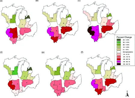
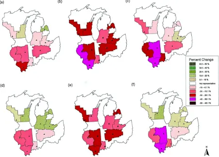
Long-season maize in all future climate scenarios (Fig. 3) clearly showed decreases in yields in the southern and central locations. The decreases range from 0 to−45% as compared to yields estimated using VEMAP data. The largest decreases in yield occurred in western Illinois for all future climate scenarios. In contrast, the northern locations showed increases in yields under these same future climate scenarios. In the four northernmost agricultural areas (east cen-tral Michigan, southwest Michigan, eastern Wiscon-sin, and western Wisconsin) increases in maize yield ranged from 0.1 to 45% as compared to yields using VEMAP data. An exception to this pattern was for the HadCM2-GHG scenario with doubled variance, where southwestern Michigan and western Wisconsin had−0.1 to −10% decreases in yield. The doubled variability runs of both scenarios resulted in extreme decreases in yield in the southern locations, and less significant increases in yield in the northern locations as compared to unchanged or halved variability runs. The greatest gains in yield occurred in the halved vari-ability scenarios because the occurrence of very low or zero yields decreased substantially in the halved variability scenarios.
Medium-season maize yields (Fig. 4) showed dra-matic decreases in yields as compared to VEMAP, even in the northern agricultural areas of the study region. Under the HadCM2-GHG and HadCM2-SUL scenarios all regions experienced decreases in yields of maize, ranging from−15.1 to−40%. In these sce-narios, no locations experienced increases in yield. Under the doubled and halved variability scena-rios, however, the northern most locations showed lesser decreases in yield and even some increases. Val-ues ranged from−30 to 20% for the halved variability scenarios, and from−40 to 15% for the doubled vari-ability scenarios. It must be noted that the actual (sim-ulated) yields obtained for medium-season maize are usually higher than those obtained for longer-season maize for all climate scenarios (Table 3). However, when compared to the current VEMAP yields as a percentage change the yields frequently decrease.
J. Southworth et al. / Agriculture, Ecosystems and Environment 82 (2000) 139–158 149
Fig. 3. Percent change in mean maximum decadal yield for long-season maize, compared to VEMAP yields, for (a) halved variability HadCM2-GHG, (b) HadCM2-GHG, (c) doubled variability HadCM2-GHG, (d) halved variability HadCM2-SUL, (e) HadCM2-SUL, and (f) doubled variability HadCM2-SUL.
5.1 to 35%. This difference in pattern may be due to different factors than the changes in yield of medium and long-season maize, perhaps related to the strong east-west precipitation gradient or differences in soils at this location.
3.2. Mean maximum decadal yield versus planting dates
The impact of changing climate on planting dates in terms of the mean maximum decadal yields (Figs. 3–5) illustrates that under future climate change scenarios later planting dates produced higher yields. In almost all cases (Table 3) the highest mean maxi-mum decadal yield occurs at a later planting date under future climate change, which explains why
medium-season maize varieties frequently have higher total yields than the longer season maize. The later planting dates for all maize varieties have the most beneficial impact on medium-season maize. The pro-ductivity induced shift to later planting dates is past the current optimal planting dates for longer season varieties and into the medium-season maize optimal planting dates. Such delays in planting dates also have been found by other researchers under future climate change scenarios (Jones et al., 1999).
3.3. Spring freezes
Fig. 4. Percent change in mean maximum decadal yield for medium-season maize, compared to VEMAP yields, for (a) halved variability HadCM2-GHG, (b) HadCM2-GHG, (c) doubled variability HadCM2-GHG, (d) halved variability HadCM2-SUL, (e) HadCM2-SUL, and (f) doubled variability HadCM2-SUL.
will increase (Fig. 6). This implies that increased frost tolerance is not an important issue for future climate change and maize growth as initially expected.
4. Discussion
4.1. Crop yield changes by region
The future climate scenarios, with increased tem-peratures and precipitation, resulted in significantly altered maize yields, at each of the 10 agricultural areas in the study region.
Across the southern areas yields generally decreased due to the daily maximum temperatures
becoming too high and hence, resulting in yield decline. Western Illinois had yield decreases of−10 to −50% for long-season maize, −10 to −40% for medium-season maize, and −10 to +40% for short-season maize. For short-season maize western Illinois was the only location with yield increases, although these increases only occurred under the HadCM2-SUL scenarios and the halved variability HadCM2-GHG scenario, i.e. the less extreme cli-mates. Eastern Illinois had yield decreases of−10 to
J. Southworth et al. / Agriculture, Ecosystems and Environment 82 (2000) 139–158 151
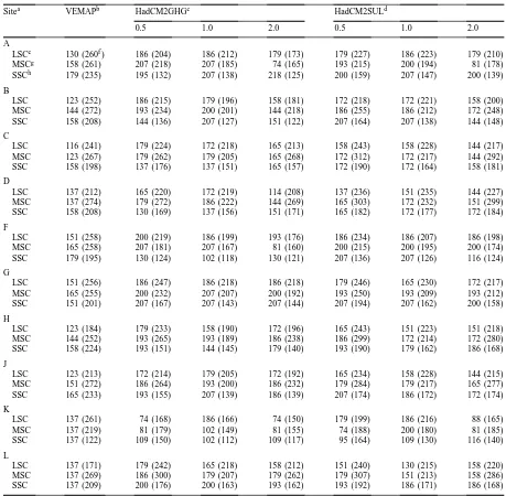
Table 3
Mean maximum decadal yield planting dates (Julian days) under VEMAP current climate and future HadCM2GHG (halved variability (0.5)/unchanged variability (1.0)/doubled variability (2.0)) and HadCM2SUL (halved variability (0.5)/unchanged variability (1.0)/doubled variability (2.0)) climate scenarios for maize varieties
Sitea VEMAPb HadCM2GHGc HadCM2SULd
0.5 1.0 2.0 0.5 1.0 2.0
A
LSCe 130 (260f) 186 (204) 186 (212) 179 (173) 179 (227) 186 (223) 179 (210) MSCg 158 (261) 207 (218) 207 (185) 74 (165) 193 (215) 200 (194) 81 (178) SSCh 179 (235) 195 (132) 207 (138) 218 (125) 200 (159) 207 (147) 200 (139) B
LSC 123 (252) 186 (215) 179 (196) 158 (181) 172 (218) 172 (221) 158 (200) MSC 144 (272) 193 (234) 200 (201) 144 (218) 186 (255) 186 (212) 172 (248) SSC 158 (208) 144 (136) 207 (127) 151 (122) 207 (164) 207 (138) 144 (148) C
LSC 116 (241) 179 (224) 172 (218) 165 (213) 158 (243) 158 (228) 144 (217) MSC 123 (267) 179 (262) 179 (205) 165 (268) 172 (312) 172 (217) 144 (292) SSC 158 (198) 137 (176) 137 (151) 165 (157) 172 (190) 172 (164) 158 (181) D
LSC 137 (212) 165 (220) 172 (219) 114 (208) 137 (236) 151 (235) 144 (227) MSC 137 (274) 179 (272) 186 (222) 144 (269) 165 (303) 172 (232) 151 (299) SSC 158 (208) 130 (169) 137 (156) 151 (171) 165 (182) 172 (177) 172 (184) F
LSC 151 (258) 200 (219) 186 (199) 193 (176) 186 (234) 186 (207) 186 (198) MSC 165 (258) 207 (181) 207 (167) 81 (160) 200 (215) 200 (195) 200 (174) SSC 179 (195) 130 (124) 102 (118) 130 (121) 207 (136) 207 (126) 116 (124) G
LSC 151 (256) 186 (247) 186 (218) 186 (218) 179 (246) 165 (230) 172 (217) MSC 165 (255) 200 (232) 207 (207) 200 (192) 193 (250) 193 (209) 193 (212) SSC 151 (201) 207 (167) 207 (143) 207 (144) 207 (194) 207 (162) 200 (158) H
LSC 123 (184) 179 (233) 158 (190) 172 (196) 165 (243) 151 (223) 151 (218) MSC 144 (252) 193 (265) 193 (189) 186 (238) 186 (299) 172 (214) 172 (280) SSC 158 (224) 193 (151) 144 (145) 179 (140) 193 (190) 179 (162) 186 (168) J
LSC 123 (213) 172 (214) 179 (205) 172 (192) 165 (234) 158 (228) 144 (215) MSC 151 (272) 186 (264) 193 (200) 186 (232) 179 (284) 179 (217) 165 (277) SSC 165 (233) 193 (155) 207 (139) 186 (139) 207 (174) 186 (172) 172 (174) K
LSC 137 (261) 74 (168) 186 (166) 74 (150) 179 (199) 186 (216) 88 (165) MSC 137 (219) 81 (179) 102 (149) 81 (155) 74 (188) 200 (180) 81 (185) SSC 137 (122) 109 (150) 102 (112) 109 (117) 95 (164) 109 (130) 116 (140) L
LSC 137 (171) 179 (242) 165 (218) 158 (212) 151 (240) 130 (215) 158 (220) MSC 137 (269) 186 (300) 179 (207) 179 (262) 179 (307) 151 (213) 158 (286) SSC 137 (209) 200 (176) 200 (163) 193 (162) 193 (192) 186 (171) 186 (168) aA: eastern Illinois; B: east-central Indiana; C: north-west Ohio; D: south-central Michigan; F: southern Illinois; G: south-west Indiana; H: eastern Wisconsin; J: south-west Wisconsin; K: western Illinois; and L: Michigan thumb.
bVEMAP dataset for current climate data.
cHadCM2GHG is the Hadley Center data for 2050–2059 from the greenhouse gas only run. dHadCM2SUL is the Hadley Center data for 2050–2059 from the greenhouse gas and sulphate run. eLSC: long-season maize.
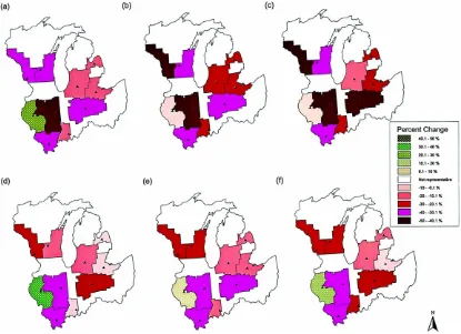
Fig. 5. Percent change in mean maximum decadal yield for short-season maize, compared to VEMAP yields, for (a) halved variability HadCM2-GHG, (b) HadCM2-GHG, (c) doubled variability HadCM2-GHG, (d) halved variability HadCM2-SUL, (e) HadCM2-SUL, and (f) doubled variability HadCM2-SUL.
J. Southworth et al. / Agriculture, Ecosystems and Environment 82 (2000) 139–158 153
Results were very consistent across climate scenar-ios. Southwest Indiana yields decreased between 0 and −20% for long-season maize, 0 and −30% for medium-season and short-season maize. East-central Indiana had yield decreases of −10 to −30% for long-season maize, 0 to −30% for medium-season maize, and−20 to−50% for short-season maize.
Agricultural areas in the northern states of the study region typically experienced more increased yields under the six future climate scenarios, especially for long-season maize. Northwest Ohio had yield changes of+10 to−20% for long-season maize,+20 to−30% for medium-season maize, and 0 to −30% for short-season maize. South-central Michigan yield changes ranged from +20 to −10% for long-season maize,+20 to−20% for medium-season maize, and
−10 to−30% for short-season maize. The Michigan thumb area experienced the greatest yield increases for long-season maize, with+20 to+50% increases above current yields, for medium-season maize+20 to−30% changes in yield, and 0 to−30% decreases for short-season maize. Southwest Wisconsin had
+20 to−10% changes in yield for long-season maize,
+10 to−30% for medium-season maize, and−20 to
−50% changes for short-season maize. Finally, east-ern Wisconsin, had yield changes of 0 to +40% for long-season maize,+20 to−30% for medium-season maize, and−10 to−40% for short-season maize.
The results across all 10 agricultural areas have some significant and consistent patterns. The two main patterns are (1) short-season maize has low yields compared to current yields under changed cli-mate scenarios except in western Illinois, and (2) the halved variability climate scenarios produced both the highest maize yield increases and some of the lowest decreases in agricultural areas in the southern states, indicating that changes in future climate variability, producing more extreme climatic events, will be detri-mental to future agricultural production. Hence, as this research illustrates, it is extremely important to model both changes in mean and variability of future climate. Our results indicate that the currently grown (pre-dominant) maize hybrid (long-season maize) will have increased or better yields under future climate conditions, compared to current yields, than will the medium and short-season maize hybrids. How-ever, in terms of actual yield, medium-season maize yields are frequently greater than those obtained from
longer-season maize for the same climate scenario due to the later planting dates under climate change. Short-season maize does not appear to be as viable under changed climate conditions across the study region.
Spatially, results show that the agricultural areas in the northern states (southwest Wisconsin, eastern Wisconsin, south-central Michigan, northwest Ohio, and the Michigan thumb) will experience increases in maize yields as a result of climate change, while those in the southern and central regions (western Illi-nois, eastern IlliIlli-nois, southern IlliIlli-nois, southwest In-diana, and east-central Indiana) will show a clearly decreasing trend. The more extreme climate scenario, as represented by HadCM2-GHG, results in greater reduction of maize yields than HadCM2-SUL. The HadCM2-GHG scenario produces mean monthly sum-mer temperatures that are 1–4◦C warmer than the HadCM2-SUL scenarios. Increased surface air tem-peratures result in a reduction in agricultural produc-tivity in many crops due to earlier flowering and a shortening of the grain-fill period. The shorter the crop duration, the lower yield per unit area (Lal et al., 1998), as is seen in results in central and southern locations in the study region. However, in northern locations of the study area, where low temperatures currently limit the grain fill period, increases in temperatures due to climate change will result in the grain filling period lengthening and increased yields.
4.2. Daily maximum temperatures
High temperatures affect agricultural production directly through the effects of heat stress at critical phenological stages in the crop’s growth. In maize, high temperatures at the stages of silking or tassel-ing result in significant decreases in yield. Both the CERES-maize and another crop model, EPIC, use the temperature-sum approach to calculate developmen-tal time, where GDD=[(Tmax−Tmin)/2]−Tbase.
In the case of the EPIC model, the only condition is that GDD cannot be<0. This has an important impli-cation for climate change studies, because increasing the daily mean temperature in the EPIC model will never directly slow the developmental rate. In the case of CERES-maize, if the maximum daily temperature (Tmax) is above 44◦C or the minimum daily
average 3-h temperature is calculated for eight peri-ods of the day using an interpolation scheme. If this 3-h temperature is greater than the base temperature or <44◦C, then the 3-h temperature contributes to the daily temperature to be summed. In addition, if the 3-h temperature is >34◦C, then the developmental rate is assumed to decrease. Using the CERES-maize model, when the maximum daily temperature exceeds 44◦C, then the developmental rate will be slowed due to high temperatures. In addition, if the amplitude of daily temperature fluctuations increases to the extent that the maximum daily temperature is exceeding 44◦C or the minimum daily temperature is less than the base temperature, the developmental rate will de-crease, even if the mean daily temperature stays the same. In contrast, with the standard GDD approach, such as that used in the EPIC model, only the mean daily temperature effects developmental time, not the amplitude of daily temperature. Again, this has implications for climate change studies, where daily temperature amplitude may change as the climate changes (Riha, 1999; personal communication). This inclusion of both the amplitude and the mean
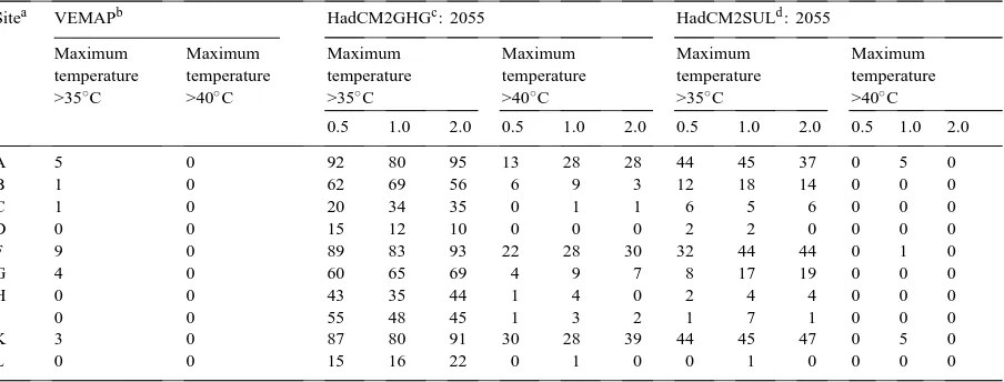
temper-Table 4
Number of days in the growing season (1 May–30 September) with maximum daily temperatures 35.0–39.9◦C, and 40.0–44.9◦C under VEMAP current climate and future HadCM2GHG (halved variability (0.5)/unchanged variability (1.0)/doubled variability (2.0)) and HadCM2SUL (halved variability (0.5)/unchanged variability (1.0)/doubled variability (2.0)) climate scenarios for the year 2055
Sitea VEMAPb HadCM2GHGc: 2055 HadCM2SULd: 2055
Maximum
aA: eastern Illinois; B: east-central Indiana; C: north-west Ohio; D: south-central Michigan; F: southern Illinois; G: south-west Indiana; H: eastern Wisconsin; J: south-west Wisconsin; K: western Illinois; and L: Michigan thumb.
bVEMAP dataset for current climate data.
cHadCM2GHG is the Hadley Center data for 2050–2059 from the greenhouse gas only run. dHadCM2SUL is the Hadley Center data for 2050–2059 from the greenhouse gas and sulphate run.
ature is an important reason for the selection of the CERES-maize model.
Using regression analyses, Rosenzweig (1993) found that daily maximum temperatures greater than 33.3◦C in July and August were negatively corre-lated with maize yield in the US Maize Belt and that daily maximum temperatures >37.7◦C caused severe damage to maize. The future climate scenarios used had maximum daily temperatures >35◦C on several days during July and August (Table 4). Results in this table match closely with yield changes with an increased number of days with temperatures greater than 35◦C within a given climate scenario, resulting in decreased yields.
J. Southworth et al. / Agriculture, Ecosystems and Environment 82 (2000) 139–158 155
The US Environmental Protection Agency (EPA) found a decrease in maize yields under conditions of future climate change of 4–42% due to tempera-tures rising above the range of tolerance for the maize crops (EPA, 1998). Saarikko and Carter (1996) found that the thermal suitability for spring wheat in Fin-land could shift northwards by 160–180 km per 1◦C increase in mean annual temperature. In areas of cur-rent growth the timing of crop development under a warmer climate shifts to earlier in the year, thus short-ening the development phase, resulting in decreased yields. In northwest India, Lal et al. (1998) found a re-duction of 54% in wheat yields with a 4◦C rise in mean daily temperatures. Using a doubled atmospheric CO2
concentration (720 ppmv) from present day and a 5◦C rise in mean daily temperatures, the decrease in yield was only 32% from current conditions. These results are similar in terms of pattern and trend to those of this research, with increasing summer maximum tem-peratures resulting in decreased yields.
4.3. Impacts of CO2fertilization
This approach, using the CERES-maize model, enables us to model the predicted future climate, and CO2levels based on this future climate, and to
eval-uate the crop response. This research used a future atmospheric CO2 concentration of 555 ppmv,
com-pared to 360 ppmv for current conditions. For maize, a C4 crop, this response is not as important as for C3 crops such as soybeans. C4 crops are more efficient photosynthetically than C3 plants and show less re-sponse to increasing atmospheric CO2 concentration,
which provides a future potential agricultural adapta-tion of C3 crops over C4 crops due to their enhanced growth functions with higher concentrations of CO2
(Rosenzweig and Hillel, 1998; Rosenzweig, 1993). Assessment of both the effects increased atmospheric CO2 concentrations and climatic change impacts on
agricultural production is a crucial area of research because the two factors occur together.
4.4. Climate variability impacts on maize yields
The halved variability climate scenarios produced maize yields with the greatest increases in yield for long-season maize. In addition, decreases in yield for
the agricultural areas in the southern states, and for the medium-season and short-season maize varieties were much less extreme. These results were expected for the halved variability scenarios which resulted in less extreme events, e.g. fewer spring freezes (Fig. 6) and a decreased number of extreme temperature events (Table 4).
The doubled climate variability scenarios repre-sent the most extreme climate scenarios modeled. In addition, a doubling of current or future variability conditions is probably at the maximum limit of likely changes in climate variability. As such, these doubled variability scenarios probably represent the most ex-treme variability changes that might occur by 2050. Under the doubled variability scenarios, particularly the doubled variability HadCM2-GHG scenario, the greatest decreases in maize yields for long-season maize are found. Medium-season and short-season maize also experience large decreases in yield under these scenarios. The doubled variability scenario also results in highly variable year-to-year variability in maize yields across the 10 years modeled and studied. These results are in accordance with those found by other research groups, and are not surprising given the high incidence of days with extreme temperatures, compared to the halved variability scenarios (Table 4). When evaluating all six future climate scenarios in terms of their impacts on midwestern maize yields it is quite evident that the most detrimental agricultural impacts would arise from a future climate similar to the HadCM2-GHG doubled variability scenario.
but not for SIRIUS which had no change) across all sites, which was related to an increased number of days at sub-optimal temperatures. For the same loca-tions Semenov and Barrow, (1997) found that when changes in climate variability are included in a climate change analysis the results found are quite different. For wheat yields, a decrease in yield of 20% was ob-served when variability was doubled. Again, these re-sults are similar to those reported in this research.
4.5. Potential adaptations to climatic change
Another important area of research concerns pos-sible adaptation strategies to climate change and the effects of those strategies. The most obvious adapta-tions identified in this research are (1) the develop-ment of a more heat tolerant hybrid of long-season maize and (2) switching from maize (a C4 crop) to soybeans (a C3 crop) to take advantage of increased atmospheric CO2concentrations promoting increased
growth and greater tolerances for hot temperatures (although how realistic this may be will be dependent on market factors). In fact, increased heat tolerance in short and medium-season maize varieties may provide the opportunity to manipulate planting dates of these hybrids and provide adaptation equal or superior to adaptation of long term varieties under some condi-tions, which is illustrated by the use of shorter season maize varieties rather than sorghum in recent years in the southwestern United States. Under increased climate variability and increased extreme events, soil moisture management will become more critical and will require improved soil infiltration and water hold-ing capacity. Tillage and cropphold-ing systems that yield these benefits will increase in economic value to farmers. Also, there will be increased concern about soil erosion with more extreme rain events, especially if agricultural program standards for conservation compliance that limits erosion are tightened.
5. Conclusions
Our primary conclusions are:
• A lengthened growing season, dominated by a cen-tral period of high maximum daily temperatures, is a critical inhibitor to maize yields. Late spring and early fall frosts do not affect maize yields.
• The north-south temperature gradient in the mid-western Great Lakes states is extremely important in influencing patterns of maize yield under future climate conditions.
• Climate variability is a significant factor influenc-ing maize yields because increased climate variabil-ity results in the largest decreases in future maize yields.
Understanding responses of individual farms to changes in mean climate and changes in climate vari-ability is essential to understanding the impacts of climate change on agriculture at a regional scale (Wassenaar et al., 1999). The research discussed here is part of a larger project examining possible farm-level adaptations to the potential changes pre-dicted from the crop modeling. Continuing research will incorporate crop modeling of soybeans (DSSAT SOYGRO) and wheat (DSSAT CERES-wheat), both in terms of the potential mean changes in future cli-mate and the potential changes in clicli-mate variability. These results will be used as inputs into the Purdue Crop Linear Program (PC/LP) model for farm level decision analysis. The results from the DSSAT mod-els (CERES-maize, CERES-wheat, and SOYGRO) flow into PC/LP, then as management/economic de-cisions change the type of production, results are fed back into the crop model for further adjustment to crop production modeling. This will allow the devel-opment of farm level strategies to be created and then tested by running back through the model scenarios with the adaptations incorporated.
The approach taken in this research examines adap-tation at the farm level. Other research has examined agricultural response to climate change primarily on a regional or national basis. Both are important. How-ever, at the local level, climate change research must include the full spectrum of climate, soils, biology, management, and economics if there is to be any link between analysis and reality. This research hopes to provide the basis for strategic planning and risk man-agement by farmers and the agricultural infrastructure to better adapt to changing conditions.
Acknowledgements
J. Southworth et al. / Agriculture, Ecosystems and Environment 82 (2000) 139–158 157
Program of the United States Environmental Pro-tection Agency. We thank Dr. David Viner for his help and guidance with the use of the HadCM2 data, which was provided by the Climate Impacts LINK1 Project (DETR Contract EPG 1/1/68) on behalf of the Hadley Center and the United Kingdom Meteorologi-cal Office. We thank Dr. Joe Ritchie at Michigan State University for his help and advice on CERES-maize throughout this project and Dr. Susan Riha at Cornell University for her comments on the temperature sen-sitivity of CERES-maize. We thank Dr. Timothy Kit-tel at the National Center for Atmospheric Research (NCAR), Boulder, Colorado for recommendations, help and guidance with VEMAP data acquisition and use. We greatly appreciate the assistance of Dr. Linda Mearns at NCAR in discussions on climate variability and for her comments regarding this manuscript and our research. We thank Michael R. Kohlhaas for his help with editing earlier versions of this manuscript. Finally, we thank the participants in the IPCC GCTE Focus 3 Conference, held in Reading, UK, Septem-ber 1999, for wonderful discussions and insightful comments and questions.
References
Adams, R.A., Hurd, B.H., Reilly, J., 1999. Agricultural and Global Climate Change: A Review of the Impacts to US Agricultural Resources. On-Line Pew Report at http://www.pewclimate. org/projects.
Adams, R.M., Rosenzweig, C., Peart, R.M., Ritchie, J.T., McCarl, B.A., Glyer, J.D., Curry, R.B., Jones, J.W., Boote, K.J., Allen Jr., L.H., 1990. Global climate change and US agriculture. Nature 345, 219–224.
Barrow, E., Hulme, M., Semenov, M., 1996. Effect of using diff-erent methods in the construction of climate change scenarios: examples from Europe. Clim. Res. 7, 195–211.
Carnell, R.E., Senior, C.A., 1998. Changes in mid-latitude vari-ability due to increasing greenhouse gases and sulphate aerosols. Clim. Dyn. 14, 369–383.
Chiotti, Q.P., Johnston, T., 1995. Extending the boundaries of climate change research: a discussion on agriculture. J. Rural Stud. 11, 335–350.
Dhakhwa, G.B., Campbell, C.L., LeDuc, S.K., Cooter, E.J., 1997. Corn growth: assessing the effects of global warming and CO2 fertilization with crop models. Agric. For. Meteorol. 87, 253– 272.
Environmental Protection Agency (EPA), 1998. Climate Change and Indiana. Office of Policy, EPA 236-F-98-007g.
1LINK homepage at http://www.cru.uea.uk/link/.
Harrison, P.A., Butterfield, R.E., 1996. Effects of climate change on Europe-wide winter wheat and sunflower productivity. Clim. Res. 7, 225–241.
Hoogenboom G., Tsuji, G.Y., Pickering, N.B., Curry, R.B., Jones, J.J., Singh, U., Godwin, D.C., 1995. Decision support system to study climate change impacts on crop production. In: Climate Change and Agriculture: Analysis of Potential International Impacts. ASA Special Publication No. 59, Madison, WI, USA, pp. 51–75.
Hulme, M., Barrow, E.M., Arnell, N.W., Harrison, P.A., Johns, T.C., Downing, T.E., 1999. Relative impacts of human-induced climate change and natural climate variability. Nature 397, 688– 691.
IPCC (Intergovernmental Panel on Climate Change), 1990. First assessment report. In: Houghton, J.T., Jenkins, G.J., Ephraums, J.J. (Eds.), Scientific Assessment of Climate Change — Report of Working Group I. Cambridge University Press, UK. IPCC (Intergovernmental Panel on Climate Change), 1995. Second
assessment report — climate change. In: Houghton, J.T., Meira Filho, L.G., Callender, B.A., Harris, N., Kattenburg, A., Maskell, K. (Eds.), The Science of Climate Change. Cambridge University Press, UK.
Jones, J.W., Jagtap, S.S., Boote, K.J., 1999. Climate change: implications for soybean yield and management in the USA. In: Kaufman, H.E. (Ed.), Proceeding of World Soybean Research Conference VI, August 4–7, 1999, Chicago. University of Illinois, Urbana-Champaign, IL. pp. 209–222.
Kaiser, H.M., Riha, S.J., Wilks, D.S., Sampath, R., 1995. Adap-tation to global climate change at the farm level. In: Kaiser, H.M., Drennen, T.E. (Eds.), Agricultural Dimensions of Global Change. St. Lucie Press, FL, USA, pp. 136–152.
Kane, S., Reilly, J., Tobey, J., 1992. An empirical study of the economic effects of climate change on world agriculture. Clim. Change 21, 17–35.
Katz, R.W., Brown, B.G., 1992. Extreme events in a changing climate: varibility is more important than averages. Clim. Change 21, 289–302.
Kittel, T.G.F., Rosenbloom, N.A., Painter, T.H., Schimel, D.S., Fisher, H.H., Grimsdell, A., VEMAP Participants, Daly, C., Hunt Jr., E.R., 1996. The VEMAP phase I database: an integrated input dataset for ecosystem and vegetation modeling for the conterminous United States. CDROM and World Wide Web (URL=http://www.cgd.ucar.edu/vemap/).
Lal, M., Singh, K.K., Rathore, L.S., Srinivasan, G., Saseendran, S.A., 1998. Vulnerability of rice and wheat yields in NW India to future changes in climate. Agric. For. Meteorol. 89, 101–114. Liang, X., Wang, W., Dudek, M.P., 1995. Interannual variability of regional climate and its change due to the greenhouse effect. Glob. Plan. Change 10, 217–238.
Mavromatis, T., Jones, P.D., 1998. Comparison of climate change scenario construction methodologies for impact assessment studies. Agric. For. Meteorol. 91, 51–67.
Mearns, L.O., Rosenzweig, C., Goldberg, R., 1997. Mean and variance change in climate scenarios: methods, agricultural applications, and measures of uncertainty. Clim. Change 35, 367–396.
Mearns, L.O., Rosenzweig, C., Goldberg, R., 1996. The effect of changes in daily and inter-annual climatic variability on Ceres-wheat: a sensitivity study. Clim. Change 32, 257–292. Mearns, L.O., Katz, R.W., Schneider, S.H., 1984. Extreme
high-temperature events: changes in their probabilities with changes in mean temperature. J. Clim. Appl. Meteorol. 23, 1601–1613. Nafziger, E.D., 1994. Corn planting date and plant population. J.
Prod. Agric. 7, 59–62.
Pearce, F., 1997. State of the Climate — A Time for Action. WWF Report.
Peiris, D.R., Crawford, J.W., Grashoff, C., Jeffries, R.A., Porter, J.R., Marshall, B., 1996. A simulation study of crop growth and development under climate change. Agric. For. Meteorol. 79, 271–287.
Phillips, D.L., Lee, J.J., Dodson, R.F., 1996. Sensitivity of the US corn belt to climate change and elevated CO2: I. Corn and soybean yields. Agric. Syst. 52, 481–502.
Rind, D., 1991. Climate variability and climate change. In: Schlesinger, M.E. (Ed.), Greenhouse-Gas-Induced Climate Change: A Critical Appraisal of Simulations and Observations. Development in Atmospheric Science 19, Elsevier, New York. Rosenburg, N.J., 1992. Adaptation of agriculture to climate change.
Clim. Change 21, 385–405.
Rosenzweig, C., 1993. Modeling crop responses to environmental change. In: Solomon, A.M., Shugart, H.H. (Eds.), Vegetation Dynamics and Global Change. Chapman and Hall, NY, USA. Rosenzweig C., Hillel, D., 1998. Climate Change and the Global Harvest: Potential Impacts of the Greenhouse Effect on Agriculture. Oxford University Press, New York.
Rosenzweig, C., Hillel, D., 1993. Agriculture in a greenhouse world. Natl. Geograph. Res. Explor. 9, 201–221.
Saarikko, R.A., Carter, T.R., 1996. Estimating the development and regional thermal suitability of spring wheat in Finland under climatic warming. Clim. Res. 7, 243–252.
Semenov, M.A., Barrow, E.M., 1997. Use of a stochastic weather generator in the development of climate change scenarios. Clim. Change 35, 397–414.
Semenov, M.A., Wolf, J., Evans, L.G., Eckersten, H., Iglesias, A., 1996. Comparison of wheat simulation models under climate change. II. Application of climate change scenarios. Clim. Res. 7, 271–281.
Smith, J.B., Tirpak, D.A. (Eds.), Appendix C: Agriculture in The Potential Effects of Global Climate Change on the United States. US Environmental Protection Agency, Washington, DC, 1989.
Thornton, P.K., Bowen, W.T., Ravelo, A.C., Wilkens, P.W., Farmer, G., Brock, J., Brink, J.E., 1997. Estimating millet production for famine early warning: an application of crop simulation modeling using satellite and ground based data in Burkina Faso. Agric. For. Meteorol. 83, 95–112.
United States Department of Agriculture (USDA), 1997. Intera-gency agricultural projections committee. Agricultural Baseline Projections to 2005, Reflecting the 1996 Farm Act. Staff Report WAOB-97-1. World Agricultural Outlook Board, Office of the Chief Economist, Washington, DC.
Wassenaar, T., Lagacherie, P., Legros, J.P., Rounsevell, M.D.A., 1999. Modelling wheat yield responses to soil and climate variability at the regional scale. Clim. Res. 11, 209–220. Wolf, J., Evans, L.G., Semenov, M.A., Eckersten, H., Iglesias, A.,