Penggunaan Perangkat Lunak untuk Simulas

(1)

Disini kita bisa mengggunakan perangkat lunak untuk

penyelesaian masalah Sinyal-Sistem dengan bahasa pemrograman seperti:

- C

- Delphi

- Java

- Matlab

- Matcad

- dll

Penggunaan Perangkat Lunak untuk Simulasi

Kita pilih salah satu

dalam pelatihan ini

(2)

(3)

(4)

Perintah Help

> > help sin

SI N Sine.

SI N(X) is the sine of the elements of X.

(5)

1. Memulai suatu operasi aritmatika

Menghitung volume pada suatu bola dengan jari-jari r= 2.

Anda ingat bahwa persamaan matematik untuk volume suatu bola dengan jari-jari r adalah:

Volume = (4/ 3)

π

r3

Anda dapat menyelesaikan dengan mengetik seperti berikut:

(6)

(7)

3. Bentuk Input

r= 0;

while r< 10

r= input('Masukkan nilai radius: ');

if r< 0,break,end

vol= (4/ 3)* pi* r^ 3;

fprintf('Volume= % 7.3f\ n',vol)

end

(8)

(9)

5. Membuat Fungsi

Buat fungsi demof_.m dengan mengetik seperti berikut: function y= demof_(x)

y= (2* x.^ 3 + 7* x.^ 2 + 3* x-1)./ (x.^ 2-3* x + 5* exp(-x));

Untuk memanggilnya: x= 0: 1: 10;

y= demof_(x); y

Buat fungsi kedua sbb:

function [ mean,stdv] = mean_stdv(x) n= length(x);

mean= sum(x)/ n;

stdv= sqrt(sum(x.^ 2)/ n-mean.^ 2);

(10)

6. Membuat Grafik

% File Name: graph_1.m n= 201;

delx= 10/ (n-1); for k= 1: n

x(k)= (k-1)* delx;

y(k)= sin(x(k))* exp(-0.4* x(k)); end

% plot(x,y)

plot(x,y,'linewidth',4)

title('Grafik yang pertama') xlabel('x'); ylabel('y');

(11)

Membuat Grafik Polar

% File Name: graph_3.m t= 0: 0.05: pi+ 0.1;

y= sin(3* t).* exp(-0.3* t); polar(t,y)

(12)

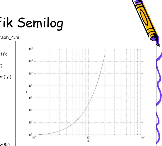
Grafik Semilog

% File Name: graph_4.m t= .1: .1: 3;

x= exp(t);

y= exp(t.* sinh(t)); loglog(x,y)

% semilogy(x,y) grid

(13)

Grafik dua fungsi

% File Name: graph_5.m x= 0: 0.05: 5;

y= sin(x); plot(x,y) hold on z= cos(x); plot(x,z,'--')

title('Penggambaran dua fungsi bersamaan') xlabel('sumbu x'); ylabel('y(x) dan z(x)')

(14)

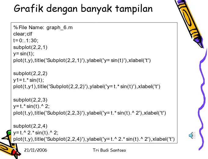
% File Name: graph_6.m

plot(t,y1),title('Subplot(2,2,2)'),ylabel('y= t.* sin(t)'),xlabel('t')

subplot(2,2,3) y= t.* sin(t).^ 2;

plot(t,y),title('Subplot(2,2,3)'),ylabel('y= t.* sin(t).^ 2'),xlabel('t')

subplot(2,2,4)

y= t.^ 2.* sin(t).^ 2;

(15)

(16)

% File Name: graph_7.m clear,clf

x_title= -2: .2: 2; y_title= -2: .2: 2;

[ x,y] = meshgrid(x_title,y_title); z= x.* exp(-x.^ 2-y.^ 2);

mesh(x,y,z)

title('3-D plot of z= x.* exp(-x.^ 2-y.^ 2)') xlabel('x'); ylabel('y'); zlabel('z');

(17)

21/11/2006 Tri Budi Santoso

% Create the figure

fig = figure('Units' , 'points' , 'Position', [ 30 30 380 230] );

% Create the axes and make it so they are cleared when clicked on ax = axes('Units' , 'points', ...

'Position' , [ 30 15 200 200] , ... 'ButtonDownFcn', 'cla');

% Change the viewing angle and cause subsequent plots to be placed % on the same axes

view(3) hold on

% Create the uicontrol pushbuttons

String = { 'Close' , 'Membrane' , 'Peaks' } ;

Call = { 'close(gcf)' , 'cla; surf(membrane)' , 'cla; surf(peaks)' } ; for lp= 1: 3,

ui(lp) = uicontrol('Style' , 'pushbutton', ... 'Units' , 'points', ...

% Notice you will get simple_gui1.m and simple_gui1.mat % To load the figure, type simple_gui1

% To save this figure to an M-file that can be called to recreate the GUI , % you can use either the line

% print(gcf,'-dmfile','simple_gui1') % or

(18)

(19)