ESTIMATION OF TREE POSITION AND STEM DIAMETER USING SIMULTANEOUS
LOCALIZATION AND MAPPING WITH DATA FROM A BACKPACK-MOUNTED LASER
SCANNER
J.Holmgren1∗
, H.M.Tulldahl2, J.Nordlöf2, M.Nyström1, K.Olofsson1, J.Rydell2, E. Willén3
1 Dept. of Forest Resource Management, Swedish University of Agricultural Sciences, Umeå, Sweden
-(johan.holmgren,mattias.nystrom,kenneth.olofsson)@slu.se
2 Electrooptical Systems and Sensor Informatics, Swedish Defence Research Agency, Linköping, Sweden
-(michael.tulldahl,jonas.nordlof,joakim.rydell)@foi.se
3 Swedish Forest Research Institute, Uppsala, Sweden - [email protected]
Commission III, WG III/1
KEY WORDS:Mobile laser scanning, Forest inventory, Tree detection, Tree map, SLAM, Remote sensing
ABSTRACT:
A system was developed for automatic estimations of tree positions and stem diameters. The sensor trajectory was first estimated using a positioning system that consists of a low precision inertial measurement unit supported by image matching with data from a stereo-camera. The initial estimation of the sensor trajectory was then calibrated by adjustments of the sensor pose using the laser scanner data. Special features suitable for forest environments were used to solve the correspondence and matching problems. Tree stem diameters were estimated for stem sections using laser data from individual scanner rotations and were then used for calibration of the sensor pose. A segmentation algorithm was used to associate stem sections to individual tree stems. The stem diameter estimates of all stem sections associated to the same tree stem were then combined for estimation of stem diameter at breast height (DBH). The system was validated on four 20 m radius circular plots and manual measured trees were automatically linked to trees detected in laser data. The DBH could be estimated with a RMSE of 19 mm (6%) and a bias of 8 mm (3%). The calibrated sensor trajectory and the combined use of circle fits from individual scanner rotations made it possible to obtain reliable DBH estimates also with a low precision positioning system.
1. INTRODUCTION
Forest inventories are still conducted using manual measurements on sample plots. However, there is now a rapid development of sensors which can produce point clouds of 3D measurements and automate the process of forest inventory. Measurements from mobile systems covering larger areas will better capture the tree size variation compared to manual measurements or static sys-tems. The position estimates for Mobile Laser Scanning (MLS) systems are usually obtained through a combined use of an in-ertial measurement unit (IMU) and a Global Navigation Satel-lite System (GNSS). Supporting data from GNSS are needed in order to avoid drifts of the estimates from the IMU. However, using MLS systems in environments with blocked or multi-path satellite signals requires additional data in order to obtain a stable system. One solution is to use Simultaneous Localization And Mapping (SLAM) algorithms which use laser scanner data from surrounding objects to estimate the sensor position. These al-gorithms are usually efficient for indoor applications with well-defined planar surfaces in many directions but the problem be-comes more difficult in outdoor environments. However, some algorithms have recently been developed that efficiently use the geometry of the traversed surroundings, both indoor and in out-door environments, without the need of high precision inertial measurements (Bosse et al., 2012, Zhang and Singh, 2014). The system presented in this study consists of (1) a positioning system for an initial estimate of the sensor trajectory, (2) a laser scanner operated with multiple lasers each separated with different an-gles relatively the horizontal plane of the scanner, (3) algorithms
∗Corresponding author
for correction of the initial sensor trajectory using laser measure-ments of surrounding objects (dynamic calibration), and (4) al-gorithms for estimates of tree positions and stem diameters. The objective was to develop algorithms for forest inventory that can use low precision IMU data as input and will work in difficult forest environments.
2. METHODOLOGY
2.1 Experimental MLS system
The MLS system consists of the units: positioning system, laser scanner, and a computer for system control and data logging. The laser scanner was a Velodyne VLP 16 which emits approximately 300 000 pulses per second using 16 lasers each rotating 360 de-grees in the horizontal plane and are separated by two dede-grees relatively to the scanner’s horizontal plane, symmetrically allo-cated on both sides of the scanner’s horizontal plane. The scanner was tilted backwards in order to also receive laser returns on the ground near the scanner (Figure 1).
2.2 Positioning system
Figure 1. Experimental MLS system.
2.3 Estimation of the sensor trajectory
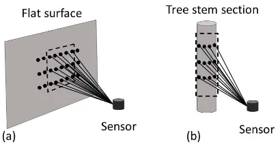
The system requires an initial estimate of the trajectory that is corrected with the laser scanner data using the dynamic calibra-tion algorithm. The dynamic calibracalibra-tion builds on previous devel-opments where Inertial Navigation System (INS) measurements were corrected using a ground height model and the laser scan-ner was mounted on a small UAV system (Tulldahl and Larsson, 2014, Tulldahl et al., 2015). The dynamic calibration adjusts the information of sensor pose from the initial estimate given by the stereo-camera to a calibrated pose using the laser scanner data. The dynamic calibration is performed in two steps; the first step adjusts the position based on data from one scanner revolution (each 0.1 s), and the second step based on data over a 1 s time interval. The first step corrects for short-time drift while the sec-ond step, comprising more laser data, corrects for long-time drift. For the dynamic calibration we extract features from the laser data. These features consist of two types: tree stem sections (SS) and flats (F). Stem sections correspond to 3D-laserdata returned from the stem-part of the trees. Flats correspond to 3D-laserdata returned from flat surfaces, which mainly comprise parts of the ground in the forest environment. A modification of the c-value proposed by Zhang et al. (2014) was used in order to find laser re-turns from flat areas and stem sections. The basic principle used for extracting SS and F are the same. For both features we cal-culate the local 3D-point variation from an ideal flat surface in a surrounding kernel from each 3D-point. High local variation indicates that the 3D-point comes from e.g. a bush, branches, or other small object. These points are rejected and not used for the dynamic calibration. 3D-points with a surrounding of low local variation are put on a stack for further examination. The difference for detecting SS and F is in the shape of the kernel describing the surrounding (neighbors) to each 3D-point. For the detection of flats, we use a kernel which approximately cor-responds to a square when projected to a surface perpendicular to the laser optical axis. For the detection of stem sections, we use a kernel which corresponds to an elongated rectangle, when projected onto objects. The concept is schematically illustrated (Figure 2). The stack of F and SS features is further examined with respect to quality measures. For F the quality measure is the surface roughness (RMSE of 3D-points from a plane fitted to the points), and for SS the quality measure is the RMSE of the 3D-points in relation to circles fitted to the 3D-point data. The circle fit also estimates stem diameter and stem center position which are further used in the processing. The extracted features
were used to solve the correspondence and matching problems. The best quality features of both F and SS obtained from a scan-ner revolution is used for calibration of the sensor pose versus the features obtained from earlier scanner revolutions. For opti-mization of the best pose in 6 DOF (degrees of freedom) (x, y, z, roll, pitch, yaw), we use two different distance metrics. For F, we minimize the to-plane distance, and for SS both the point-to-plane (to the stem surface) distance and the point-to-line dis-tance (to the estimated stem center position). The first dynamic calibration step was used to reduce short-time errors of the initial sensor trajectory. However, also a small drift becomes a problem if the same location is measured after some time because multi-ple estimates are then obtained for each tree. The solution was to aggregate stem sections for longer time intervals in order to have initial tree position estimates (simple trees). These simple trees were processed in time sequential order. To account for small residual position errors, the features from 10 scanner revolutions were aggregated and the sensor position further corrected to re-duce accumulated errors over longer time intervals. In this second calibration step, more F and SS features are available and these are used to fine tune the pose in relation to the calibrated fea-tures from previous scanner revolutions. A search was first done for feature neighbors within a search distance in the horizontal plane (1 m). A weighted average was formed for the position in the plane using all available neighbors within the search dis-tance. The pairs with position and weighted averages of neighbor position values were used for an estimate of a rigid body trans-formation in the horizontal plane for each (1 s) time interval. The transformation was applied for all flats and stem sections within the time interval. The altitude values were also corrected with a similar procedure (z-correction) after corrections in the horizon-tal plane.
Figure 2. Schematic illustration of the kernel (dashed line) used for detection of flat surfaces (a) and stem sections of a tree (b). The kernel defines a neighborhood of 3D-points (illustrated by
black dots) collected by the laser scanner sensor.
2.4 Stem segmentation
This procedure was repeated until no more stem sections could be added to the current start segment. A stem section that was added to a stem segment was also removed from the list of avail-able stem sections. A new segment was then formed starting with the next available stem section from the list. This procedure was repeated until all stem sections had been added to a stem segment.
2.5 Estimation of tree position and stem diameter
A fine-tune of the horizontal position estimates of stem sections was performed based on the results from the stem segmentation. A 3D-line was estimated from the stem sections of each segment. A pair of XY-coordinates was estimated for each stem section: (1) the original stem section position, and (2) the position where the 3D-line intersected a horizontal plane in which the original position was included. The stem sections were sorted in time order. A time interval was formed just large enough to include stem sections from at least three different stem segments. A rigid body transformation in the horizontal plane was done using the coordinate pairs within the time interval. This was repeated for sequential time intervals until all stem sections were corrected. Several stem segments could belong to the same tree after the initial segmentation, for example because of shaded areas due to branches etc. A merge of stem segments was therefore performed based on the main direction of each segment. The PCA was cal-culated using all stem section points within a segment in order to find the main direction and the deviation from the direction vec-tor was calculated. All stem segments were compared with each other. The direction vector of the longest tree stem segment in the z-direction was used. The intersection was calculated of the direction vector and the horizontal plane defined by the mean z-value for the shorter tree stem segment. The two segments were merged into one if the intersection point was within a shorter range to the mean horizontal coordinates (x, y) of the smaller segment points than the sum of the mean values of the radius from the two stem segments. A Digital Elevation Model (DEM) of the ground was created using the flats that had been used for the dynamic calibration. These points were usually located on the ground. A ground height value was estimated for each raster cell size by first selecting points within a radius of 8 m if the stan-dard deviation of the heights of these points were less than 0.5 m. The ground height value was then estimated with inverse squared distance weighting using the heights of the selected points. Val-ues were then in a second step set to raster cells without valVal-ues. For a raster cell value without value the lowest required number of steps to the side (rows, columns) was used in order to have a window that contained at least one ground height value. Inverse distance weighting was used if there were more than one raster cell with a ground height value within the window. This process was repeated for every raster cell in order to have a DEM without raster cells with missing values. It was then possible to derive the vertical distance to the ground for each stem section within a stem segment. All stem sections within a tree segment were used to estimate stem diameter at breast height (DBH, 1.3 m above ground level). A curve fitting was performed using a third de-gree polynomial (Eq. 1). In this way circle fits from individual scan revolutions could be combined to form more reliable DBH estimates.
where d= stem diameter
h= distance from the ground
3. VALIDATION
The system was validated at the Remningstorp test site in south-ern Sweden. Four field plots with 20 m radius were selected. The field plots were located in mature forest dominated by Norway spruce (Picea Abies). The tree positions were measured with a total station and marked with an identification number in the sum-mer of 2011. The DBH was then re-measured with a caliper in 2016 some weeks after the collection of MLS data. Four subplots were used on each 20 m radius field plot. Three ultrasonic trans-mitters mounted on a tripod in the center of a subplot were used to obtain three distances for each calipered tree and these dis-tances were used for trilateration calculations to obtain relative coordinates for each calipered tree. The identification number of four reference trees was recorded on each subplot. The data from reference trees were used as input to rigid body transformation in order to obtain global coordinates for each calipered tree. The spatial pattern of the local tree coordinates from the MLS system was matched with the global tree coordinates with manual mea-sured trees using an earlier developed algorithm (Olofsson et al., 2008). A tree measured with MLS was linked to a manual mea-sured tree if they were within a distance of 0.8 m from each other. A field tree that not was linked was judged to be undetected.
4. RESULTS
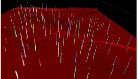
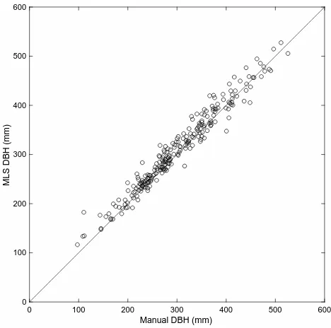
The correction of the positions of the stem sections could be val-idated by visualization the results with a 3D vrml vector model (Figure 3). The stem sections from the same tree segment were located on top of each other without much random deviations. The spatial pattern of tree positions could be used to link the trees detected with laser data with the corresponding manual measured trees (Figure 4). The DBH for the linked trees were estimated without large deviations (Figure 5). The root-mean-square-error (RMSE) and bias are presented for each field plot (Table 2). The relative values of RMSE and bias (relRMSE and relbias) were de-rived by division with the mean value of manual DBH measure-ments. The DBH was estimated for all linked trees on all plots with a RMSE of 19 mm (6%) and a bias of 8 mm (3%). All trees could not be detected and there were differences between plots in the proportion of detected trees. The sensor trajectory and the stem density were different for the plots. The DBH mean values of undetected trees were lower compared to the DBH mean value of all trees for plots except one plot on which only one tree not was detected.
Figure 4. Automatic linking of laser and manual mesaured trees on a 20 m radius field plot (brown circle). The crosses are laser
detected trees, the circles are manual measured trees, green symbols indicate linking.
0 100 200 300 400 500 600
Manual DBH (mm) 0
100 200 300 400 500 600
MLS DBH (mm)
Figure 5. Stem diameter estimates 1.3 m above ground (DBH).
5. CONCLUSIONS
The SLAM algorithm presented here was developed for tree mea-surements and could be used with data collected with low cost hardware components. Stem diameters (1.3 m above ground level, DBH) were estimated with 19 mm RMSE (relative RMSE 6%) which is similar compared to other studies where more ad-vanced hardware were used. For example, the ROAMER system including a tactical grade IMU and a FARO Photon 120 terres-trial laser scanner mounted on a six-wheeled all-terrain vehicle (ATV) was used for estimation of stem diameters on a rectangu-lar plot with sides of 74 m and 50 m in Finland. Stem diameter (DBH) was estimated with a RMSE of 24 mm (relative RMSE
Plot RMSE[mm] relRMSE[%] bias[mm] relbias[%]
1 19 5 2 1
2 24 7 12 4
3 12 5 7 3
4 19 7 10 3
Table 1. Stem diameter (DBH) estimations for linked trees on four field plots.
Plot All Omission Mean all [mm] Mean UDT [mm]
1 53 12 337 236
2 79 17 292 174
3 63 1 252 297
4 85 11 282 257
Table 2. Total number of trees (all), number of undetected trees (Omission), mean DBH for all trees (Mean all), and mean DBH
for undetected trees (Mean UDT).
8%) (Liang et al., 2014a). Also, a mobile laser scanner (AKHKA R2) with a tactical grade fiber optical IMU and FARO Focus 3D scanner was used on rectangular plot with the sides 40 m and 50 m, also in Finland. The personal laser scanner was mounted on a backpack and trees on the plot were mapped using three walking paths and stem diameter (DBH) was estimated with a RMSE of 51 mm (relative RMSE 15%) (Liang et al., 2014b). One reason for small errors despite the use of low cost hardware components in the current study could be the combined use of multiple cir-cle fits, each derived from individual scanner revolutions, using a diameter-height function (Eq. 1). Thus, the relative errors from the positioning systems over longer time will not affect the stem diameter estimates. Also, the position errors are small enough after the dynamic calibration to allow for an efficient tree stem segmentation which allow for a combined use of multiple circu-lar fits from the same tree stem.
ACKNOWLEDGEMENTS
This research was financed by Hildur and Sven Wingquist’s foun-dation for forest science research, Carl Trygger’s founfoun-dation for scientific research, Bo Rydin’s foundation for scientific research, Norrskog research foundation, Södra research foundation, and Brattås foundation for forestry research. We would like to thank Jon Söderberg and Johan Öhgren for support with data collection, and Mattias Tjernqvist for support with the z-correction.
REFERENCES
Bosse, M., Zlot, R. and Flick, P., 2012. Zebedee: Design of a spring-mounted 3-d range sensor with application to mobile map-ping.Robotics, IEEE Transactions on28(5), pp. 1104–1119.
Liang, X., Hyyppa, J., Kukko, A., Kaartinen, H., Jaakkola, A. and Yu, X., 2014a. The use of a mobile laser scanning system for mapping large forest plots.Ieee Geoscience and Remote Sensing Letters11(9), pp. 1504–1508.
Liang, X., Kukko, A., Kaartinen, H., Hyyppä, J., Yu, X., Jaakkola, A. and Wang, Y., 2014b. Possibilities of a personal laser scanning system for forest mapping and ecosystem services. Sensors14(1), pp. 1228–1248.
tree list graphs. In: Proceedings of SilviLaser 2008, 8th inter-national conference on LiDAR applications in forest assessment and inventory, Heriot-Watt University, Edinburgh, UK: Silvi-Laser 2008 Organizing Committee, Edinburgh: Forest Research, pp. 95–104.
Rydell, J. and Emilsson, E., 2012. Chameleon: Visual-inertial indoor navigation. In:Position Location and Navigation Sympo-sium (PLANS), 2012 IEEE/ION, IEEE, pp. 541–546.
Tulldahl, H. M. and Larsson, H., 2014. Lidar on small uav for 3d mapping. In: SPIE Security+ Defence, Vol. 9250, International Society for Optics and Photonics, pp. 925009–1–14.
Tulldahl, H. M., Bissmarck, F., Larsson, H., Grönwall, C. and Tolt, G., 2015. Accuracy evaluation of 3d lidar data from small uav. In:SPIE Security+ Defence, Vol. 9649, International Society for Optics and Photonics, pp. 964903–1–11.