*Corresponding author. Tel.:#46-13-28-1504; fax: #46-13-28-8975.
E-mail address:[email protected] (R.W. GrubbstroKm).
Modelling rescheduling activities in a multi-period
production}inventory system
Robert W. Grubbstro
K
m*, Ou Tang
Department of Production Economics, Linko(ping Institute of Technology, S-581 83 Linko(ping, Sweden
Received 1 April 1998; accepted 19 April 2000
Abstract
Decisions for planning production activities for multi-period production}inventory systems have been studied in a number of papers applying input}output analysis and the Laplace transform. The decisions have concerned activities spread out over time without having the opportunity to adjust future decisions when the external and/or internal circumstances change. In this paper, we extend the analysis to situations when rescheduling is possible. Firstly, di!erent classes of causes justifying rescheduling activities are presented including periodic rescheduling and `net changea.
Secondly, in terms of previously developed theory, we model the behaviour of a simple single-level production}inventory system for which its production plan may be modi"ed at one point in the future. ( 2000 Elsevier Science B.V. All rights reserved.
Keywords: Rescheduling; Laplace transform; Multi-period production}inventory system; Renewal process
1. Introduction
The purpose of a production}inventory system is to meet the external market requirement by e$-ciently using the resources in the system. In multi-level production}inventory systems, material re-quirements planning (MRP) is usually employed as an information system to connect the relationships between demand and supply of di!erent items. Starting from the master production schedule (MPS), MRP explodes detailed production deci-sions from top-level items down to the lower-level items. In several previous papers [1}5],
optimisa-tion condioptimisa-tions for producoptimisa-tion planning are derived for such systems applying input}output analysis and the Laplace transform. The production sched-ule for end items is used as the MPS. When deter-mining the MPS, safety stock considerations have been included to enhance system performance. In the theory hitherto developed, the opportunity for adjusting the production schedule due to the changed background circumstances has been disre-garded within the planning horizon.
In a real production}inventory system, when the system updates information about its operational environment and the market forecast, there may be reasons to change the previously decided produc-tion schedule, although this schedule earlier was regarded as the optimal one. Because of internal and external unforeseen developments, there can be a need to revise the schedule considerably. In
practice, this is often done either periodically, or when a strong need is experienced.
On the other hand, every rescheduling of"nished top-level items usually causes changes concerning lower-level production plans due to the e!ects from internal demand a!ected by the parts explosion. Such adjustments of plans also have an augmented e!ect in an assembly system, and this is often refer-red to assystem nervousness. Nervousness may be-come the obstacle in the implementation of MRP and even cause the collapse of the whole system. A general discussion on rescheduling and the related nervousness topic can be found in [6}9].
In this paper, we "rst review related work con-cerning the rescheduling problem in multi-level and related production}inventory systems. The basic mechanism for justifying rescheduling is discussed in an analytical framework. As a few preliminary
developments, a "rst model for rescheduling
departing from the net present value (NPV) approach is analysed. Based on this model, a num-ber of numerical examples are studied. The major part of our"ndings is summarised in a concluding section together with some ideas for developing this theory in new directions.
2. Motives for rescheduling
Rescheduling refers to the process of changing
order or operation due dates, usually as a result of their being out of phase with when they are needed
[10]. Due to an increasing uncertainty of the in-formation while the previous plan is implemented, MRP frequently needs to update unplanned events within or outside the production}inventory system in order to keep the information accurate. Unplan-ned events of these kinds are usually considered to emanate from the following four sources, which also provoke the requirement for rescheduling, namely (i) uncertainty in external demand; (ii) un-certainty in supply conditions; (iii) e!ect of a rolling planning horizon, and (iv) a`system e!ecta.
Changes in external demand conditions are very common reasons for performing rescheduling ac-tivities. Normally, the MPS is determined accord-ing to a forecasted demand and assumed supply situation, including considerations such as capacity
limitations. As soon as a customer changes his demand pattern, either quantitatively or timely, the original forecast needs to be adjusted. If the MPS is frozen and such changes are ignored, di!erences between demand and supply will develop resulting for instance in a depressed service level or an in-creased cost of holding inventory due to additional capital tied up.
Neither the supply from outside nor the internal supply of intermediate items is entirely predictable in the real world situation. There can be a variation in the vendor or production lead times, scrap can exceed estimated quantities, errors are discovered in inventory data, and machine breakdowns occur [11]. All these causes re#ect that the information on available inventory may be inaccurate. Whether or not an original MRP plan should continue to be implemented, depends on how to remedy the prob-lem by rescheduling and the economic conse-quences thereof.
The third motive for initiating a new schedule is the rolling planning horizon. Blackburn et al. [12] discussed the horizon sensitivity embedded in many dynamic lot-sizing algorithms. When the time of planning moves forward, new demand ap-pears, which causes changes in part, if not all of the previous MPS. A forward lot-sizing rule such as the Silver-Meal algorithm, can diminish the horizon sensitivity by accumulating the changes near to the end of the horizon. However, such an algorithm usually misses the optimal solution. Studies of ner-vousness and lot-policy relationships can also be found in [13}15]. Besides traditional lot-sizing rules, we also observe that other optimal produc-tion planning procedures, for example when using the net present value (NPV) approach [2], are sensitive to the planning horizon. The MPS always faces a pressure to be rescheduled when time is rolling forward.
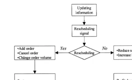
Fig. 1. Trade-o!between di!erent rescheduling decisions.
This is what is called `MRP nervousnessa. This
nervousness leads to increased costs, it reduces pro-ductivity, it lowers the service level and it creates
general states of confusion on the shop#oor [16].
Nervousness is probably the main obstacle against considering rescheduling opportunities.
3. Methods for rescheduling
Orlicky [17] pointed out that there are two essential methods for updating information
and rescheduling in an MRP system. The "rst is
`schedule regenerationa and the second is `net
changea.
According to the American Production and Inventory Control Society, regeneration is de"ned to be a process approach in which the master production schedule is totally re-exploded down through all bills-of-materials, to maintain valid priorities [10]. New requirements and planned or-ders are completely recalculated and regenerated at that time. One obvious advantage of this method is that it purges errors that have accumulated in the system so that the system information becomes more accurate. Since it concerns all elements in the system, a good solution can be obtained. On the other hand, regeneration is limited by its frequency due to the computational e!orts involved and their corresponding cost.
A `net changea is an approach in which the
material requirements plan is continually retained in the computer. Whenever a change is needed in requirements, open order inventory status, or bill-of-materials, a partial explosion and netting is made for only those parts a!ected by the change. Therefore, all irrelevant items are left untouched. The calculation e!ort in this case is smaller. Orlicky [17] and Oden et al. [18] mentioned that net change might cause more nervousness because it results in a high frequency of many minor changes, and sometimes a rescheduling has to be made to a recently rescheduled plan.
Most MRP software packages include both methods. Net change is applied more frequently to update information on a continuous basis while regeneration is applied in a longer time interval to refresh the whole system.
As mentioned in the previous section, the purpose of rescheduling is to"ll the gap between the forecasting information and the actual state. Therefore, the service level of the system is expected to increase and inventory costs are reduced. Never-theless, the negative result from rescheduling is that it creates nervousness. Fig. 1 illustrates that there is
a trade-o!between the rescheduling and opposite
non-rescheduling (stay) alternatives.
Carlson et al. [13] discussed the cost of ner-vousness. Since a production plan is less sensitive to the change of order volume or to cancel an order, they concentrated on the cost of scheduling a new setup. The cost is then supposed to be a function of time. If the rescheduled setup is moved backwards beyond the minimum lead time, the cost is in"nitely large. In other intervals, they proposed using a sim-ilar estimation procedure as for the usual setup cost to obtain a rescheduling cost. However, we may note that their nervousness cost is based on the limitations of a single-level item system. The chain e!ect of nervousness was ignored because of its complexity. Van der Sluis [19] also stated that the nervousness cost is determined by the early replen-ishments, which cause all scheduled replenishments to be moved forward. This follows the same frame-work as of Carlson et al. but Van der Sluis focused on a multi-level system.
performance of the whole system and the moral reaction of the sta!involved.
Instead of investigating the trade-o!between res-cheduling decisions in monetary terms, some re-searchers have put e!ort into studying dampening mechanisms for stabilising system nervousness. Ho [21] suggested a dampening"lter to be used to screen out insigni"cant rescheduling messages which de-pend on the decision criterion used in the"lter, such as limitation of time changes and the cost of ner-vousness. Penlesky et al. [22] compared four
di!er-ent "ltering heuristics for rescheduling. All these
heuristics perform statistically better than the"xed due-date procedure (no rescheduling) and dynamic procedure (frequent rescheduling). A similar study was also carried out by Christy and Kanet [23]. In short, the advantage to accomplish rescheduling un-der appropriate circumstances is obvious.
From our literature review, we have noticed that most research carried out has been based on simu-lation methodology when studying the reschedul-ing problem. Analytical models appear only to have been presented by Inderfurth [20], in which he studied the impact on the stability of production planning from di!erent parameters in inventory
control rules, such as from the (s,S) and (s,nQ)
policies. The objective function thus applied mea-sured the stability of the system rather than in-cluded economic consequences.
4. Basic problem
Our basic problem treated is how to determine the appropriate circumstance for when and when not to reschedule. In other words, what is to trigger the act of rescheduling. Essentially, we envisage that there are two main approaches. The "rst is a time trigger, like regeneration and net change taking place at regular pre-determined points in time. The frequency is determined in advance and the production}inventory system may be inspected periodically to examine if there is a need or not to reschedule. The second approach is that a state of the system reached automatically triggers a res-cheduling activity. Information concerning such a state may be the inventory or backlog situation or how much the actual demand has departed from
its previous forecast, etc. Similar two classes of policies are studied in basic inventory theory with periodic-review models and reorder-point systems. Apart from limiting ourselves to a single-level system, in our treatment to follow, we also con"ne ourselves to a case in which there is only one point of time in the future at which we can reconsider a previously decided production plan. Hence, we avoid complications from recurring rescheduling opportunities. These limitations will be relaxed in future studies since analysing multi-level produc-tion}inventory systems is our main target. We also assume that the horizon of the original plan (the length of the time interval covered initially) does not change at the time a new schedule is made, i.e. we are not considering a rolling planning process. This enables the possibility of a comparison be-tween rescheduling or not. If and when the schedule is changed, it concerns the remaining part of the original horizon. As in previously developed the-ory, demand will be assumed to follow a stochastic renewal process.
As mentioned in Section 3, the cost from carrying out a rescheduling operation is di$cult to deter-mine in practice. For our purpose we assume that there is a"xed exogenously determined cost asso-ciated with deciding to reschedule.
At"rst, let us introduce the following notation.
The predetermined point in time at which a
pre-viously determined plan can be revised is ¹, the
sequence of production decisions prior to this point
in time are denotedpand those at and beyond this
point are denotedp@.
Letdand d@ represent dependent stochastic
se-quences of a demand process, before and after the
possible rescheduling time ¹. Assume that these
have probability distributions written dF(z) and
dF@(uDz), respectively, meaning that the probability
of an outcomed@"umight possibly depend on the outcome of the previous sequenced"z.
The general framework for rescheduling is illus-trated in the diagram in Fig. 2. At time 0, we make
decisions for productionpandp@based on demand
sequencesdandd@. At the rescheduling point, we calculate the expected net present value with and without rescheduling and make a comparison.
Fig. 2. Decision-tree diagram for rescheduling.
are realised. The notationp
irefers to di!erent
pos-sible choices ofp, and d
j to di!erent possible
out-comes of d, and similarly for p@
l and d@k. For
expository reasons, the "gure assumes that there exist "nite sets of opportunities for choosing the production decisions and for demand outcomes, but in our treatment below this limitation is not
required. The symbol in the "gure refers to
a`tollaamounting to the economic consequences
from making a new schedule. Thestay optionrefers
to the opportunity to stick to the originally decided plan for the period succeeding the rescheduling point. The decision to reschedule is immediately followed by a choice of new planp@
l.
Let NPV(p,p@Dd,d@) be the stochastic economic outcome, based on these four sequences. The objec-tive function to be maximised is assumed to be the expected value
E(NPV(p,p@Dd,d@))
"
PP
NPV(p,p@Dz,u) dF@(uDz) dF(z). (1)A "rst basic question addressed, is whether there
exist simple conditions concerning the function NPV(p,p@Dd,d@) in order for the "rst part of the
decision sequence p to be optimal irrespective of
whether there is an opportunity to choose a new second part of the sequence p@ at ¹after the "rst
outcomedhas been revealed, or not.
We compare the two cases after introducing the abbreviationsx"p,y"p@and
a(x,y,z)"
P
u
NPV(p,p@Dz,u) dF@(uDz)
"
P
u
NPV(x,yDz,u) dF@(uDz). (2)
In the"rst case, both the"rst and the second part of the production decision sequencex"pandy"p@
are decided at the initial timet"0.
The optimisation problem for this case then reads
NPVH"Max
x
Max
y
P
a(x,y,z) dF(z). (3)
Let xH and yH, respectively, denote the optimal
solution.
In the second casex"pis chosen att"0 andy"
p@chosen att"¹after the outcomez"dis known. We now instead have the optimisation problem
NPVHH"Max
x
P
Max
y
a(x,y,z) dF(z). (4)
Let xHH denote the optimal solution for the "rst part of the decision sequence andyHH(z) the optimal remaining decision sequence (depending on the
outcomez) in this second case.
It is obvious that the second case in general produces a higher value of the objective function as given by the statement
NPVHH*NPVH.
If there were no cost associated with changing the plan, in general, it would always pay to make the change. You can never lose by doing this.
A major question remaining is whether or not the optimal initial decision sequence remains the same with and without the option to reschedule? In the following theorem, we show that in a speci"c case of independence between the periods, the original opti-mal sequence for both parts of the horizon remains optimal, also after the outcomezis revealed.
Theorem 1.
If L2a(x,y,z)
Hence,yHHwill be independent of the outcome z. This also implies that NPVHH"NPVH.
Furthermore, assuming a second, weaker type of independence between the two parts of the horizon, we"nd a su$cient condition for the"rst part of the decision sequence to remain optimal whether or not there are rescheduling opportunities:
Theorem 2.
If L2a(x,y,z)
LxLy ,0, then xHH"xH.
Theorems 1 and 2 provide su$cient conditions for the optimal"rst part of the decision sequence to be the same, irrespective of whether or not there are opportunities to revise the decisions. Their proofs are included in the appendix. Necessary conditions remain to be investigated.
As a simple example illustrating the rescheduling problem, we consider the following variation of the
Newsboy problem. Letx be an amount produced
initially before a stochastic demandzoccurs and let
ybe an amount which can be produced to cover
a possible backlog when zis known. Letr be the
unit revenue, c the unit production cost, K the
setup cost and c( a unit penalty for each unit sold from the second batch. Let us further assume that
z is exponentially distributed with a parameter
jand thatr'c#c(. We distinguish three intervals forzcreating di!erent expressions for total pro"ts (for simplicity written NPV):
a(x,y,z)"!c(x#y)!K(sgn(x)#sgn(y))
#
G
rz ifz(x,
rz!c((z!x) ifx)z(x#y,
r(x#y)!c(y ifx#y)z.
In the stay case, we have
NPVH"Max
x
Max
y
P
= 0
je~jza(x,y,z) dz
"Max
x
Max
y
A
r(1!e~j(x`y))!c(e~jx(1!e~jy)
j
!c(x#y)!K(sgn(x)#sgn(y))
B
which is maximised for
xH"ln(r/c)
j ,yH"0, ifK(
r!c(1#ln(r/c))
j ,
andxH"0,yH"0, otherwise.
When rescheduling is considered, we instead obtain the problem
NPVHH"Max
x
P
=0
je~jzMax
y
a(x,y,z) dz.
The inner maximisation has the solution
yHH"
G
z!x ifz'x#K/(r!c!c(),0 elsewhere.
Inserting this function and developing the integral gives us
NPVHH
"Max
x
A
r(1!e~jx)#(r!c!c()e~j(x`K@(r~c~c())
j
!cx!K
B
,which has the unique solution
xHH"
G
ln ((r!(r!c!c()e~jK@(r~c~c())/c)
j ifK(
r!c
j !cxHH,
0 otherwise.
Since r!(r!c!c()e~jK@(r~c~c()
(r, the
opti-mum initial production xHH is smaller for the
rescheduling alternative compared to the stay
case and with positive production xH(a smallK).
We may also note that the threshold value of K,
beyond which no production is optimal, is smaller for the stay case than for the rescheduling case, since
r!c(1#ln(r/c))
j (
r!c
j !cxHH.
5. Extension of NPV theory to cover non-zero initial net inventory
5.1. Stockout and inventory functions
The previously developed theory, in which among other questions safety stock issues have been focused upon [1,5], has treated cases when no initial inventory nor any initial backlog have been present. For treating a basic rescheduling problem, the theory needs to be extended to cover cases with opportunities for a non-zero initial net inventory. The decision sequencespandp@from Section 4 are now interpreted as sequences of batches produced
and the demand sequencesdandd@as realisations
of a renewal process, i.e. a sequence of unit demand events separated by independent stochastic time intervals.
The net inventory written R(t) is de"ned to be
R(t)"S(t)!B(t), where S(t)*0 and B(t)*0 are
inventory and stockouts, respectively, andR(t) can be either positive or negative. The relationship
be-tween expected inventory E(S(t)), expected
stock-outs E(B(t)), expected cumulative demand E(DM(t))
and cumulative productionPM is given by
E(S(t))!E(B(t))"R(0)#PM!E(DM (t)), (5)
whereR(0) is the initial net inventory. In terms of the Laplace transform, we have
E(SI(s))!E(BI(s))"R(0)
s #PMI(s)!E(DMI(s)), (6) where the tildes denote transforms of the
corre-sponding time functions. The symbolsis used for
the complex Laplace frequency.
In previous papers, for instance [2], the stockout function has been developed in terms of the trans-form for demand following a renewal process, as-sumingR(0)"0:
E(BI(s))" fI P
M`1
s(1!fI )"E(DMI(s))!
1 s
PM
+ j/1
fI j, (7)
which holds for time intervals during which PM is
constant. Here fI(s) is the transform of the density function of the time between two consecutive
de-mand events. In the case that R(0)#PM*0, we
immediately obtain the generalisation
E(BI(s))"fI R(0)`P
M`1
s(1!fI) "E(DMI(s))!
1 s
R(0)`PM
+ j/1
fI j. (8)
WhenR(0)#PM(0, we instead have
E(BI(s))"E(DMI)!R(0)#PM
s . (9)
Therefore, for the appropriate intervals during whichPM is given:
E(BI(s))"
G
fIR(0)`PM`1s(1!fI )
"E(DMI )!1
s
R(0)`PM
+ j/1
fI j, R(0)#PM*0,
E(DMI)!R(0)#PM
s , R(0)#PM(0.
(10)
Similarly, we obtain the expected inventory func-tion
E(SI(s))
"
G
R(0)#PM
s !
f(1!fIR(0)`PM)
s(1!fI ) , R(0)#PM*0,
0, R(0)#PM(0.
(11)
5.2. Objective function and optimisation conditions
As shown in previous papers, for instance [3], the net present value of the cash#ow in this system can easily be presented in terms of the Laplace transform. By ignoring a possible lost sales event at the end of the horizon, the expected Net Present Value for the backlogging case can be written
NPV"r[E(DI(o))!oE(BI(o))#B(0)]
!+n
k/1
(K#c(PMk!PMk~1))e~otk, (12)
wherer,c,Kandoare the given parameters being
the unit sales price, the unit production cost, the "xed setup charge and the continuous interest rate,
respectively. We always assume thatr'c,
other-wise there would never be any chance of making a pro"t from the production. Cumulative produc-tion is a staircase function described by the level
PM
LE(BI(s))
LPMk "[E(BI(w))]PMk`1![E(BI (w))]PMk
"1
2pi
P
b`i=
w/b~i=
([E(BI(w))]
PMk`1![E(BI(w))]PMk)
e~(s~w)tk!e~(s~w)tk`1
s!w dw
"
G
!1
2pi:bw`i/b~=i=
fIR(0)`PMk`1
s
e~(s~w)tk!e~(s~w)tk`1
s!w dw, R(0)#PMk*0,
!1
2pi:bw`i/b~=i= 1 s
e~(s~w)tk!e~(s~w)tk`1
s!w dw, R(0)#PMk(0.
(15) constitutes the production decisions to be taken.
The termoE(BI(o)) accounts for delayed payments from backlogging andB(0) is the initial stockout at
time t"0. The objective function NPV is to be
maximised subject to constraints of the types
PM
k`1'PMk'0 and tk`1'tk*0, for k"1,
2,2,n, wherenis the total number of batches until
the horizon.
Because cumulative productionPM
k is a staircase
function, the expected stockouts E(BI(o)) in the above equation are the sum of£~1ME(BI(s))N multi-plied by impulses of unit height and of a duration restricted to each interval (the characteristic func-tion). This multiplication in the time domain is equivalent to a convolution in the frequency do-main. Therefore,
E(BI(s))"+n
k/0
[E(BI(s))]
PMk*e~st
k!e~stk`1
s
" 1
2pi
n + k/0
P
b`i=
w/b~i=
[E(BI(w))]
PMk
]e~(s~w)tk!e~(s~w)tk`1
s!w dw, (13)
where the asterisk denotes the convolution
opera-tion and where b is real and chosen so that the
integral converges. By convention, we let t
0"0
andPM0"0. The time derivative is
LE(BI(s))
Lt
k
"e~stk[[E(B(t
k))]PMk~1![E(B(tk))]PMk] (14)
and the di!erence with respect to PM
k (being
inte-ger-valued) is
SinceE(DI(o)) andB(0) in the objective function are independent of the decision variablest
kandPMk, the
necessary optimisation conditions thus read
LNPV
Rt k
"oe~otk(!r([E(B(t
k))]PMk~1![E(B(tk))]PMk)
#(K#c(PM
k!PMk~1))))0, (16) LNPV
LPM k "!ro([E(BI (o))]PMk`1![E(BI(o))]PMk)
!c(e~otk!e~otk`1))0, (17)
fork"1, 2,2,n.
For the "rst batch time we have the weak
in-equalityt
1*0, whereas for later timestk'0, for
k*2, which create equalities in Eq. (16). The
complementarity conditions for the"rst time there-fore requires
LNPV
Lt
1
t
1"0. (18)
5.3. Initial net inventory cases
The initial net inventory, either as an inventory or a stockout, has an impact on the production plan following. When there is an initial backlog,
which means that R(0)(0 and B(0)'0, the
fol-lowing theorem for the system applies.
Theorem 3. The optimal xrst batch PM1 is at least
B(0), i.e. PM1*B(0), or PM1#R(0)*0. This means
that any initial backlog is immediately covered by the
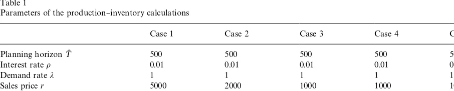
Table 1
Parameters of the production}inventory calculations
Case 1 Case 2 Case 3 Case 4 Case 5
Planning horizon¹K 500 500 500 500 500
Interest rateo 0.01 0.01 0.01 0.01 0.01
Demand ratej 1 1 1 1 1
Sales pricer 5000 2000 1000 1000 1000
Fixed setup costK 100 100 100 300 600
[image:9.544.28.481.527.618.2]Variable production costc 100 100 100 100 100
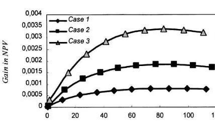
Fig. 3. Relative gain in NPV discounted to time t"¹ vs. rescheduling time¹for Cases 1}3.
Regarding conditions for the"rst batch time to be positive or zero, we have results given by the following theorem.
Theorem 4. (a)If the revenue from the initial stockout is larger than the total cost of the xrst batch,
rB(0)'K#cPM
1,there is a requirement for an
im-mediate setup, t
1"0. (b) If initial stockout B(0) is
less thanK/(r!c),we must always wait for thexrst setup, i.e. t1'0.Hence, if thexrst setup is immedi-ate, i.e. t
1"0,then we must haveB(0)*K/(r!c).
We also easily "nd that t
1'0 implies
PM1*r(B(0)!K)/c. However, we have not yet been
able to "nd su$cient conditions for an immediate setup expressed only in terms of the production parametersK,c,rando.
The results above are used for determining the optimal future production plan when choosing the rescheduling alternative. Proofs are given in the appendix.
6. Numerical examples
Based on the rescheduling problem stated in Section 4, we calculate the value from rescheduling in the following "ve examples. First we release a production plan att"0 according to the initial net inventory situation. At the rescheduling point
¹, we then compare the di!erence between the
expected future NPV for the rescheduling and stay
alternatives calculated from t"¹ and onwards.
External demand is assumed to follow a Poisson process. The stay alternative is based on initial
decisions assuming no rescheduling to be possible
(the xH solution in Section 4). The rescheduling
decisions are determined based on prior batch deci-sions and the backlog at¹(the functionyHH(xHH,z) in Section 4). The comparisons made thus implicitly assume that the optimal initial decisions are equal
(xHH"xH) irrespective of the opportunity to
res-chedule. The parameter values chosen for the pro-duction}inventory system are listed in Table 1.
When choosing di!erent alternative points at which the production plan can be revised, the cal-culations show that the value from rescheduling
increases with the rescheduling time¹in case the
time discount factor e~oT is disregarded
Fig. 4. Relative gain in NPV discounted to time t"¹ vs. rescheduling time¹for Cases 3}5.
[image:10.544.268.480.50.163.2]Fig. 5. Relative gain in NPV discounted to timet"0 vs. res-cheduling time¹for Cases 1}3.
Fig. 6. Relative gain in NPV discounted to timet"0 vs. res-cheduling time¹for Cases 3}5.
Fig. 7. The NPV vs. net inventory for the rescheduling and stay alternatives. For negative net inventories belows
1and positive net inventories aboves
2 it is advantageous to reschedule.
a maximum point for the NPV gain in di!erent cases. However, Figs. 5 and 6 indicate that the maximum point is insensitive with respect to the
parametersrandK.
Even though the expressions for the optimisation conditions are complicated, the numerical example shows that its NPV is quite linear with respect to the net inventory at¹(Fig. 7). This linearity might suggest that there is an independence of a kind that would justify the assumptionxH"xHH.
A zero net inventory generates the lowest NPV. For a positive net inventory, the NPV of the stay alternative is almost constant (slightly increasing). This means that additional initial inventory does not have an obvious impact on the expected stock-out. On the other side, for a negative net inventory, when making it more and more negative, NPV will "rst increase but approaches a constant level for very high backlogs. For small stockout levels at
t"¹, the NPV di!erence is marginal between the
rescheduling and stay alternatives. This is due to the insigni"cant di!erence in the optimum res-cheduling and stay production decisions (staircase function) for a small stockout.
If we include a rescheduling cost in the model (c@in Fig. 7), the size of the gap between the NPV of the rescheduling and stay alternatives determines an interval, outside of which it is advantageous to revise the plan. Consequently, the boundary gaps determine the states that should trigger a res-cheduling.
From the numerical example, we also notice that
the"rst batch time of the new schedule tends
to-wards zero when the initial stockout is high enough. When this"rst batch time is zero, the steps of the resulting staircase function (PMk#R(0),t
k) are
[image:10.544.30.244.217.338.2] [image:10.544.271.478.218.338.2]"nding the boundary value of the initial stockout for the"rst batch to be zero is imperative. Never-theless, this su$cient condition still needs to be further investigated as mentioned in Section 5.
7. Summary
This paper aims to take a "rst glance at the
rescheduling problem in a production}inventory system based on our previous research. After a lit-erature review of related topics, we designed a gen-eral model for addressing the rescheduling problem in the single-level case. The gap between the res-cheduling and stay alternatives can be calculated from the model and can be compared with an exogenously determined rescheduling cost.
By relaxing the initial inventory constraints in the previous NPV theory, we have also obtained some insights into the impact of the initial net inventory level on the optimal production plan. The optimal production decision for the"rst batch, especially the"rst batch time, is important in a res-cheduling study. So far as we know, this will also constitute the main constraint for the rescheduling of lower-level items in a multi-level extension. However, the su$cient conditions for an immedi-ate setup still cannot be expressed only in terms of the production parameters such asK,c,r,o. It also depends onPM1, which is a decision variable in the system. This should be an important problem to be solved in a future study.
Our discussion in Section 4 has shown su$cient conditions for the optimal solutionsxHandxHHto coincide. However, in general, the optimal decision sequences before the rescheduling point are di!er-ent for the cases with and without rescheduling options. Even in a simple case, as the example in
Section 4 indicated, the optimal solutionsxHand
xHHare di!erent. There is therefore a strong need to investigate such conditions further.
Appendix A
Proof of Theorem 1. The general solution to
[L2a(x,y,z)]/(LyLz)"0 may be written as the sum
of two arbitrary functions having the arguments
according to a(x,y,z)"A(x,y)#B(x,z). The "rst maximisation case then reads
NPVH"Max
x
Max
y
P
(A(x,y)#B(x,z)) dF(z)
"Max
x
Max
y
(A(x,y)#
P
B(x,z) dF(z))"Max
x
(A(x,yH)#
P
B(x,z) dF(z))"A(xH,yH)#
P
B(xH,z) dF(z),and the second
NPVHH"Max
x
PA
Max
y
(A(x,y)#B(x,z)
B
dF(z)"Max
x
A
Max
y
(A(x,y)#
P
B(x,z) dF(z)B
"Max
x
A
A(x,yHH)#
P
B(x,z) dF(z)B
.Hence,yHH is determined by the same
maximisa-tion asyHand thereforeyHH"yH. Then the remain-ing maximisation with respect toxwill also be the same as before, i.e.xHH"xH.
Proof of Theorem 2. The general solution to
[L2a(x,y,z)]/(LxLy),0 may be written as the sum
of two arbitrary functions having the arguments according toa(x,y,z)"M(x,z)#N(y,z).
For the"rst maximisation case we have
NPVH"Max
x
Max
y
P
(M(x,z)#N(y,z)) dF(z)
"Max
x
P
M(x,z) dF(z)#Max
y
P
N(y,z) dF(z)
"
P
M(xH,z) dF(z)#P
N(yH,z) dF(z).For the second case we instead have
NPVH"Max
x
PA
M(x,z)#Max
y
"Max
x
P
M(x,z) dF(z)#
P
Maxy
N(y,z) dF(z)
"
P
M(xHH,z) dF(z)#P
N(yHH(z),z) dF(z).Therefore, the maximisation with respect toxin the two cases coincide and xHH"xH, whereas this is not true in the general case concerning the maxi-misation with respect toy.
Proof of Theorem 3. We assume the converse, namely thatPM1#R(0)(0. Then from Eq. (15) we have
LNPV
LPM1 "!ro([E(BI(o))]PM1`1![E(BI(o))]PM1)
!c(e~ot1!e~ot2)
"!ro
A
! 12pi
P
b`i=
w/b~i=
1
o
]e~(o~wo)t1!!e(o~w)t2
w dw
B
!c(e~ot1!e~ot2)
"ro
A
Reso/0
1
o
e~(o~w)t1!e~(o~w)t2
o!w
B
!c(e~ot1!e~ot2)
"ro
A
1o(e~ot1!e~ot2)
B
!c(e~ot1!e~ot2)"(r!c)(e~ot1!e~ot2)'0.
This contradicts the optimisation condition (17). Hence, it pays to increasePM1inde"nitely as long as
PM1#R(0)"PM1#B(0)(0. Therefore, in the
opti-mum we must have PM1*B(0), meaning that the
"rst batch at least must cover the initial backlog.
Proof of Theorem 4. SincefI j(s)/sis the transform of a cumulative probability distribution with no jumps, it always holds that £~1MfIj(s)/sN*0 and that lim
t?0£~1MfI j(s)/sN"lims?= s fI j(s)/s, for allj.
For a system with an initial stockout, we have
R(0)(0. Then
LNP<
Lt
1
"oe~ot1(!r[E(B(t
1))]PM0
![E(B(t
1))]PM1)#K#cPM1)
"oe~ot1
A
!rA
[E(DM)]#B(0)!
A
[E(DM)]!£~1G
1s
PM1~B(0)
+ j/1
fI j
HBB
#K#c(PM1!PM0)
B
"oe~ot1
A
!rA
B(0)#£~1G
1s
PM1~B(0)
+ j/1
fI j
HB
#K#cPM1
B
)oe~ot1(!rB(0)#K#cPM1).
Hence, ifK#cPM
1(rB(0) thenLNPV/Lt1(0 and
from Eq. (18) t
1"0. From Theorem 3, we have
PM
1*B(0). Therefore, if K'(r!c)B(0), it must
hold thatt1'0.
When instead B(0)"0, which means R(0)*0,
the derivative is evaluated as
LNPV
Lt1 "oe~ot1
A
!rA
!£~1G
1 s
R(0) + j/1
fI j
H
#£~1
G
1s
R(0)`PM1
+ j/1
fI j
HB
#K#cPM1B
.Then, by Theorem 3 we obtain
LNPV
Lt
1
K
t/0"o(K#cPM1)*o(K#cB(0))'0,
which contradicts the optimisation condition Eq. (16). Therefore,t
1'0.
References
[2] R.W. GrubbstroKm, Stochastic properties of a production-inventory process with planned production using trans-form methodology, International Journal of Production Economics 45 (1996) 407}419.
[3] R.W. GrubbstroKm, A net present value approach to safety stocks in planned production, International Journal of Production Economics 56&57 (1998) 213}229.
[4] R.W. GrubbstroKm, A net present value approach to safety stocks in a multi-level MRP system, International Journal of Production Economics 59 (1998) 361}375.
[5] R.W. GrubbstroKm, O. Tang, Further developments on safety stocks in an MRP system applying Laplace trans-forms and input}output methodology, International Jour-nal of Production Economics 60&61 (1999) 381}387. [6] D.C. Steel, The nervous MRP system: How to do battle,
Production and Inventory Management 14 (4) (1975) 83}89. [7] H. Mather, Reschedule the reschedules you just res-cheduled: Way of life for MRP, Production and Inventory Management 18 (1) (1977) 60}79.
[8] J.R. Mini"e, R.A. Davis, Survey of MRP nervousness issues, Production and Inventory Management 17 (3) (1986) 111}120.
[9] J.R. Mini"e, R.A. Davis, Interaction e!ects on MRP ner-vousness, International Journal of Production Research 28 (1) (1990) 173}183.
[10] APICS, APICS Dictionary, 8th Edition, American Pro-duction and Inventory Control Society, Falls Church, VA, 1995.
[11] R.J. Penlesky, W.L. Berry, U. WemmerloKv, Open order due date maintenance in MRP systems, Management Science 35 (5) (1989) 571}584.
[12] J.D. Blackburn, D.H. Kropp, R.A. Millen, A Comparison of Strategies to Dampen Nervousness in MRP Systems, Management Science 32 (4) (1986) 413}429.
[13] R.C. Carlson, J.V. Jucker, D.H. Kropp, Less nervous MRP systems: A dynamic economic lot-sizing approach, Man-agement Science 25 (8) (1979) 754}761.
[14] R.C. Carlson, S.L. Beckman, D.H. Kropp, The e! ec-tiveness of extending the horizon in rolling production scheduling, Decision Sciences 13 (1982) 129}146. [15] D.H. Kropp, R.C. Carlson, J.V. Jucker, Concepts, theories,
and techniques: Heuristic lot-sizing approaches for dealing with MRP system nervousness, Decision Sciences 14 (1983) 156}169.
[16] S.N. Kadipasaoglu, V. Sridharan, Alternative approaches for reducing schedule instability in multistage manufactur-ing under demand uncertainty, Journal of Operations Management 13 (1995) 193}211.
[17] J. Orlicky, Material Requirements Planning, McGraw-Hill, New York, 1975.
[18] H.W. Oden, G.A. Langenwalter, R.A. Lucier, Handbook of Material & Capacity Requirements Planning, McGraw-Hill, New York, 1993.
[19] E. Van der Sluis, Reducing system nervousness in multi-product inventory systems, International Journal of Pro-duction Economics 30&31 (1993) 551}562.
[20] K. Inderfurth, Nervousness in inventory control: Analyti-cal results, OR Spektrum 16 (1994) 113}123.
[21] C. Ho, Evaluating the impact of operating environments on MRP system nervousness, International Journal of Production Research 27 (7) (1989) 1115}1135.
[22] R.J. Penlesky, U. WemmerloKv, W.L. Berry, Filtering heu-ristics for rescheduling open orders in MRP systems, Inter-national Journal of Production Research 29 (11) (1991) 2279}2296.