1 s2.0 S0020722515001056 main

Contents lists available atScienceDirect

International Journal of Engineering Science

journal homepage:www.elsevier.com/locate/ijengsci

Effect of the interphase zone on the conductivity or diffusivity

of a particulate composite using Maxwell’s homogenization

method

Melanie P. Lutz

a,∗

_{, Robert W. Zimmerman}

b

a_{Departments of Physics and Engineering, Solano Community College, Fairfield, CA, USA} b_{Department of Earth Science and Engineering, Imperial College, London, UK}

a r t i c l e

i n f o

Article history:

Received 15 June 2015 Accepted 15 July 2015 Available online 18 August 2015

Keywords:

Micromechanics Effective conductivity Composite materials Functionally graded materials Interphase zone

Maxwell effective medium theory

a b s t r a c t

An analytical model is developed for the conductivity (diffusivity, permeability,etc.) of a ma-terial that contains a dispersion of spherical inclusions, each surrounded by an inhomoge-neous interphase zone in which the conductivity varies radially according to a power law. The method of Frobenius series is used to obtain an exact solution for the problem of a single such inclusion in an infinite matrix. Two versions of the solution are developed, one of which is more computationally convenient for interphase zones that are less conductive than the pure matrix, andvice versa. Maxwell’s homogenization method is then used to estimate the effec-tive macroscopic conductivity of the medium. The developed model is used to analyze some data from the literature on the ionic diffusivity of concrete. Use of the model in an inverse mode permits the estimation of the local diffusivity variation within the interphase, and in particular at the interface with the inclusion.

© 2015 The Authors. Published by Elsevier Ltd. This is an open access article under the CC BY license (http://creativecommons.org/licenses/by/4.0/).

1. Introduction

Most modeling of the behavior of composite materials is carried out under the assumption that the “matrix” and “inclusions” are both homogenous, and that there is a clearly defined interface between them. The usual interface conditions are that all relevant fields (traction, displacement, temperature, heat flux,etc.) are continuous across the matrix/inclusion interface. But there are many situations in which either the interface is not sharp, or else one of the two components (matrix, inclusion) has a gradient in its physical properties. For example, a binding agent is sometimes applied to the fibers in a polymer composite, so as to promote adhesion between the fiber and the matrix (Drzal, Rich, Koenig, & Lloyd, 1983). This binding agent diffuses into the matrix during the curing process, leading to a gradient in resin concentration, which in turn may lead to gradients in physical properties within the so-called “interphase zone”. Another well known and technologically important example of materials containing such interphase zones is concrete, in which the local porosity in the cement paste increases in the vicinity of the aggregate or sand inclusions, leading to a local variation of all properties that depend on porosity, such as the elastic moduli and the transport properties (Crumbie, 1994; Lutz, Monteiro, & Zimmerman, 1997).

In a seminal paper on the effective properties of materials that possess spatially-varying local properties,Kanaun and Kudryavtseva (1986) used Green’s functions to analyze the stresses and displacements in a spherically-layered inclusion,

∗ _{Corresponding author.}

E-mail addresses:Melanie.Lutz@solano.edu(M.P. Lutz),r.w.zimmerman@imperial.ac.uk(R.W. Zimmerman).

http://dx.doi.org/10.1016/j.ijengsci.2015.07.006

located in a homogeneous matrix, and subjected to uniform far-field stress. This model of an inclusion composed of thin concen-tric layers, each having its own set of physical properties, has been widely used since then, for both the calculation of effective elastic (i.e.,Hervé, 2002) and conductive (i.e.,Caré & Hervé, 2004) properties.

Another model that is often used to account for the effect of an interphase zone can be traced back to another early paper byKanaun (1984), on so-called “singular inclusions”. Developed originally in the context of elasticity, when translated into the context of conductivity problems, Kanaun’s method considers, for example, a very thin interphase shell that has a very high conductivity. In the limit in which the thickness of the zone goes to zero, and the conductivity becomes infinite, so that their productapproaches some constant value, the annular shell can be replaced by a “flux discontinuity” boundary condition at the interface between a homogeneous inclusion and a homogeneous matrix. The case in which the conductivity and the thickness of the interphase each go to zero, while theirratioapproaches a finite value, leads to an interface condition in which the temperature undergoes a jump discontinuity. This type of model has been used in conductivity problems by, for example,Cheng and Torquato (1997), Benveniste and Miloh (1999), Hashin (2001), andBenveniste (2012), among others.

Numerous other methods have been proposed to analyze the problem of an inclusion surrounded by a thin interphase zone. Sevostianov and Kachanov (2007), for example, considered the addition of a thin layer around a spherical inclusion, and aimed to replace this “inner sphere plus thin shell” by an equivalent homogeneous inclusion. In the limit of an infinitesimally thin shell, this led to an ordinary differential equation for the evolution of the conductivity of the equivalent homogeneous inclusion. A similar method had been applied in the elasticity context byShen and Li (2005).

The present paper will approach this problem along the lines developed byLutz and Zimmerman (1996, 2005). Instead of modeling the interphase zone as a region of finite thickness, having uniform or piecewise-uniform properties, the conductivity outside of the inclusion will be assumed to vary smoothly according to a power-law variation, approaching that of the “pure matrix” phase at far distances from the inclusion. The problem of a single such spherical inclusion subjected to an otherwise uniform external gradient can be solved exactly using the power series method of Frobenius. The effective conductivity of a material containing a dispersion of such spherical inclusions will be estimated by using Maxwell’s effective medium method to approximately account for the finite concentration of inclusions.

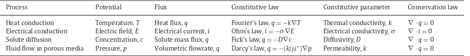
The mathematical problem of calculating the “effective conductivity” has application to numerous transport-type processes that are governed by mathematically analogous sets of constitutive and balance equations. For example, according to the classical theory of heat conduction, the heat flux is proportional to the temperature gradient, through a constant of proportionality known as the thermal conductivity. Under steady-state conditions, the divergence of the heat flux must vanish. For a homogeneous material with a piecewise-uniform thermal conductivity, this leads to a Laplace equation for the temperature. For a material with a smoothly varying thermal conductivity, the conductivity appears inside the flux term, and cannot be factored out to yield a Laplace equation (see Section2). Other physical processes that are governed by exactly analogous sets of equations include electrical conduction, ionic diffusion, and fluid flow of a slightly compressible fluid through a porous medium (Table 1).

For specificity, and since heat conduction lends itself to a simple physical interpretation and simple verbal discussion, the problem described above will be presented and solved within the context of thermal conductivity, although the results will be immediately applicable to other transport properties. The developed model will then be used to analyze some data from the literature, on the ionic diffusivity of concrete.

2. Single inclusion surrounded by a radially inhomogeneous interphase zone

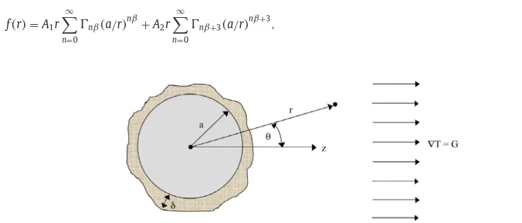
The effective thermal conductivity problem can be analyzed by solving the basic problem of an inclusion that perturbs a uniform temperature gradient of magnitudeGin an otherwise homogeneous body. A spherical coordinate system (r,

θ

,

φ

) is used, with its origin at the center of the inclusion, and thez-axis aligned with the far-field temperature gradient. The ther-mal conductivity is assumed to be a function of the radial co-ordinate,r. In the steady state, this problem is governed by (see Table 1)

∇

·[k

(

r

)

∇

T

(

r,

θ

,

φ)

]=0. (1)

Using the expression for the gradient operator in spherical co-ordinates (Arfken & Weber, 2012), Eq.(1)takes the form

1

Transport processes governed by analogous constitutive and conservation laws.

The far-field boundary conditions for the temperature are

as r→ ∞, T≈To+Gz=To+Grcos

θ

, (3)

where

θ

is the angle of inclination from thez-axis (Fig. 1).

Since the far-field temperature varies as cos

θ

, with the variable term approachingGrcos

θ

asr→ ∞, the full temperature field can be assumed to be of the formT

(

r,

θ

,

φ)

=To+f

(

r

)

cos

θ

. Insertion of this expression into Eq.(2)yields the following

differential equation forf

(

r

)

:

k

(

r

)

The thermal conductivity of the matrix is assumed to vary smoothly and monotonically with radius, and approach that of the “pure matrix” component asr→ ∞.This assumption implicitly requires that the interphase zones should be sufficiently localized so that the interphase zones of neighboring inclusions do not overlap. For most materials containing interphase zones, this is not a practical limitation. One simple but versatile function for the radial dependence of the conductivity outside of the inclusion is a constant plus a power law, as was used byTheocaris (1992)andLutz and Zimmerman (1996)to model variations in local elastic moduli:

k

(

r

)

=km+

(

ki f−km

)(

r/a

)

−β

, (5)

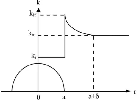
whereais the radius of the inclusion, subscriptmrefers to the “pure” matrix, and subscriptifrefers to the interface with the inclusion (Fig. 2). The exponent

β

controls the thickness

δ

of the interphase zone. If the interphase zone is defined such that the conductivity perturbation atr=a+

δ

, as given by the power law term in Eq.(5), is 10% as large as it is atr=a, it can be shown that

δ

=2.3a/β, which is to say,

β

=2.3

(

a/δ)(Lutz et al., 1997).

In order for the resulting differential equation forf

(

r

)

to be amenable to analytical treatment,

β

must be an integer.Theocaris (1992)fit power-law-type curves to the elastic moduli in an interphase zone in a set of E-glass fiber/epoxy resin composites, and found values of

β

on the order of 100.Lutz et al. (1997)found that values of

β

on the order of 20 were needed to fit the porosity gradient in the interfacial transition zone of concrete, based on data fromCrumbie (1994). Hence, restricting

β

to take on only integral values will not pose any practical limitation. As all conductive properties are closely related to the porosity, a porosity profile that can be fit by an equation of the form(5)will give rise to a conductivity profile of roughly the same form. Specifically, if one uses any effective medium theory to express the variation of, say, the thermal conductivity with porosity, and linearizes the resulting expression about the porosity of the pure matrix, a porosity profile of the form given by Eq.(5)will lead precisely to a conductivity profile having the same algebraic form.

Substitution of the conductivity variation given by Eq.(5)into Eq.(4)yields the following ordinary differential equation in the regionr>aoutside of the inclusion:

Provided that

β

is a positive integer, this equation has a regular singular point at infinity, and consequently can be solved using a Frobenius series. This equation is similar to the one that governs the elasticity problem of an inclusion with a radially inhomogeneous interphase, under far-field hydrostatic loading (Lutz & Zimmerman, 1996). Hence, the solution, which can be found through a tedious but standard procedure (Coddington, 1961), will be presented here without detailed derivation.

The general solution has the form

Fig. 2.Local variation of conductivity within and around an inclusion of radiusa. The “thickness” of the interphase zone isδ.

whereA1andA2are arbitrary constants,

Ŵ

0and

Ŵ

3are equal to 1, and the remaining non-zero

Ŵ

nare obtained from the following

recursion relationship:

Ŵ

n+β= −

ki f−km

km

[n2₊

_(β

₋₃

₎

_n−

_β

_]

(

n+

β)(

n+

β

−3

)

Ŵ

n. (8)

Application of the ratio test shows that both of the series in Eq.(7)will converge for allr>aif 0<ki f<2km,i.e.,if the

conductivity at the interface is either less than that of the pure matrix, or if it is no more than twice as high as that of the pure matrix. For cases in whichki f>2km, the resulting divergent series can be summed by applying an Euler transformation (Hinch,

1991; Lutz & Ferrari, 1993). An alternative approach that avoids the cumbersome Euler transformation, by reformulating the problem in terms of resistivity instead of conductivity, will be presented in Section4.

The general solution inside the inclusion, which is assumed to be homogeneous, is readily found from Eq.(4)to be of the form

f

(

r

)

=B1r+B2r−2. (9)

Four boundary conditions are needed in order to determine the four constants that appear in Eqs.(7) and (9). In order for the temperature to be bounded at the center of the inclusion,B2must vanish. The boundary condition at infinity, which specifies

that f

(

r

)

→Grasr→ ∞, implies thatA1=G. Continuity of the temperature at the interface between the inclusion and matrix,

wherer=a, leads to the condition

G ∞

n=0

Ŵ

nβ+A2

∞

n=0

Ŵ

nβ+3=B1. (10)

Continuity of the component of the heat flux normal to the interface, which implies continuity of the productk

(

r

)

f′

(

r

)

, leads to the condition

ki fG

∞

n=0

(

1−n

β)

Ŵ

nβ−ki fA2

∞

n=0

(

2+n

β)

Ŵ

nβ+3=kiB1, (11)

wherekiis the conductivity of the inclusion. Eqs.(10) and (11)can be solved to yield

A2= −G

₍

_k

i−ki f

)

∞

n=0

Ŵ

nβ+ki f

∞

n=0n

β

Ŵ

nβ

(

ki−ki f

)

n∞=0

Ŵ

nβ+3+ki f ∞n=0

(

n

β

+3

)

Ŵ

nβ+3

, (12)

withB1given by Eq.(10). This completes the solution to the single inclusion problem.

3. Calculation of the effective conductivity

Maxwell’s approach utilizes the leading term of the far-field temperature perturbation caused by the inclusion, and can be explained as follows. Imagine a spherical region of radiusb, containingNrandomly located identical inclusions, where in the present case each inclusion is surrounded by its own interphase zone. Each inclusion gives rise to a temperature perturbation in the far field, whose leading term is of the orderr−2_{. The total far-field perturbation due to allNinclusions is then assumed to}

simply be the sum of the perturbations due to each individual inclusion. Next, this entire spherical region of radiusbis replaced with a homogeneous region having conductivitykeff, and the temperature perturbation due to this hypothetical inclusion is

calculated. Equating the leading term of the temperature perturbation due to the “equivalent inclusion” to the leading term of the perturbation due to the collection of individual inclusions then provides an implicit equation fork_eff. For materials containing homogeneous spherical inclusions, Maxwell’s method leads to an expression forkeffthat coincides with one of the Hashin–

Shtrikman bounds, and with the predictions of Hashin’s composite sphere assemblage (Hashin, 1983).

As each of the temperature perturbation terms varies as cos

θ

, Maxwell’s method can be implemented by equating the f

(

r

)

terms. According to Eq.(7), sinceA1=G, the two leading terms in the far-field behavior offfor a single inclusion are f

(

r

)

=Gr+A2a3r−2, withA2 given by Eq.(12). Since the term Grreflects the applied temperature gradient, the

perturba-tion due to the inclusion isA2a3r−2. If there areNinclusions within the spherical region of radiusb, the total perturbation

infis given byA2Na3r−2. The perturbation infcaused by a single inclusion of radiusb, having conductivitykeff, is given by

The case in which there is no interphase zone can be recovered by settingki f=kmin Eq.(12). Since Eq.(8)shows that the

only non-zero

Ŵ

nterms will be

Ŵ

0=

Ŵ

3=1, Eq.(12)then leads toA2/G=

(

ki−km

)/(

ki+2km

)

, and Eq.(13)reduces to Maxwell’s

In the important special case of a material containing non-conductive inclusions, Eq.(16)reduces to

α

=

4. Alternative formulation for a highly conductive interphase zone

As mentioned above, the series that appear in Eq.(16)will diverge if the conductivity at the interface is more than twice as high as the conductivity of the pure matrix phase. Unfortunately, the case of a highly conductive interphase is precisely what one would expect for concrete, for example, where the excess porosity near the aggregate inclusions lead to an increased permeability, electrical conductivity, or ionic diffusivity (Shane, Mason, Jennings, Garboczi, & Bentz, 2000; Xie, Corr, Jin, Zhou, & Shah, 2015). Although these divergent series can be summed by applying an Euler transformation (Hinch, 1991), a solution containing onlyconvergentseries can be developed in these cases by formulating the problem in terms of resistivity rather than conductivity.

In terms of the resistivity

ρ

, where

ρ

=1/k, the governing equation(4)forftakes the form

ρ(

r

)

which is identical to Eq.(4), except for the changed sign in front of the term involving the derivative of the transport property. The spatial variation in resistivity can now be represented by

ρ(

r

)

=

ρ

m+

(ρ

i f−

ρ

m

)(

r/a

)

−β

Although this function is not precisely the inverse of Eq.(5)for the conductivity, it has the desired behavior at the interface with the inclusion, and at infinity, and again caused the interphase to be localized within a distance that is on the order ofa/

β

from the inclusion.

The solution to Eq.(18), with Eq.(19)used for the resistivity variation, taking into account the far-field boundary condition and the continuity conditions at the interface, is

f

(

r

)

=Gr ∞

n=0

Ŵ

nβ

(

a/r

)

nβ

+A2r

∞

n=0

Ŵ

nβ+3

(

a/r

)

nβ+3

, (20)

where

Ŵ

0=

Ŵ

3=1, and the remaining non-zero

Ŵ

coefficients are obtained from the following recursion relationship (compare

with Eq.(8)):

Ŵ

n+β= −

ρ

_{i f}−

ρ

m

ρ

m

[_n2−

(β

+3

)

n+

β

]

(

n+

β)(

n+

β

−3

)

Ŵ

n. (21)

With this new recursion relationship,A2is again found from Eq.(12), and the effective conductivity is given by Eqs.(15) and

(16), withkif=1/

ρ

if,etc. The temperature field inside the inclusion isT=To+B1rcos

θ

=To+B1z, whereB1is now found from

Eqs.(10) and (21). The series appearing in Eq.(20)will converge, for allr>a, provided that

ρ

if<2

ρ

m; in particular, these series

will converge whenever the interface ismoreconductive than the pure matrix.

5. Some numerical examples

The normalized effective conductivitykeff/km, is a function of four dimensionless parameters: the ratio of inclusion to matrix

conductivity,k_i/km; the ratio of the conductivity at the interface to the conductivity of the pure matrix,kif/km; the exponent

β

that controls the interphase thickness; and the inclusion concentration,c. The large parameter space precludes an exhaustive presentation of results. A few numerical examples will now be presented, with a brief discussion of the trends to be expected for other parameter values.

Fig. 3shows the normalized effective conductivity as a function of the inclusion concentration, for the case where the in-clusions are five times more conductive than the pure matrix, for several values of the ratiokif/km. The exponent is taken

to be

β

=10, which corresponds to an interphase zone whose thickness is about 1/8th of an inclusion diameter. The curve forkif/km=1 coincides with the Maxwell prediction for materials containing homogeneous inclusions, as well as with the Hashin–Shtrikman lower bound for a material having matrix conductivity kmand inclusion conductivityki (Hashin, 1983).

The effective conductivity increases as the interface conductivity increases, as would be expected. The deviations from the k_if/km=1 case would be smaller for larger values of

β

(i.e., for more localized interphase zones), and larger for smaller

values of

β

, although smaller values of

β

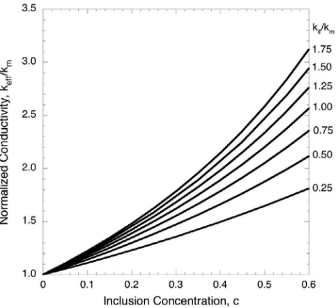
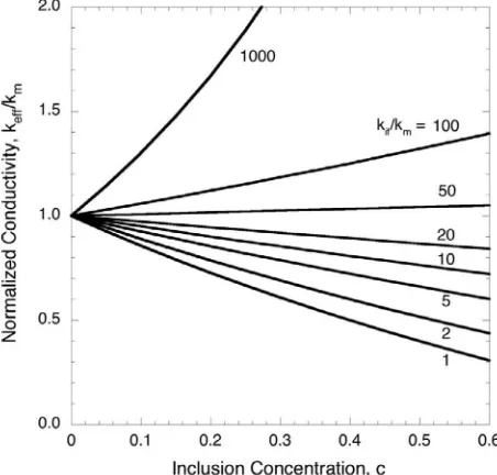
would correspond to unrealistically thick interphase zones.

An important special case is that of a material containing non-conductive inclusions, as would be the case for the permeabil-ity, diffusivpermeabil-ity, or electrical conductivity of concrete – although not the thermal conductivpermeabil-ity, since the aggregate particles are thermally conductive.Fig. 4shows the normalized effective conductivity of a material containing non-conductive inclusions, for several values of the ratiokif/km, again for the case

β

=10. The interphase zone in concrete, known as the interfacial transition

zone (ITZ), is more porous than the bulk cement paste, and so the electrical conductivity or ionic diffusivity of the interphase is expected to behigherthan that of the pure matrix.

Two competing trends are evident in this graph, as the non-conductive inclusions tend to cause the effective macroscopic conductivity to decrease, whereas the enhanced conductivity of the ITZ tends to causesk_effto increase. The curve fork_if/km=1 coincides with the classical Maxwell result for non-conductive inclusions in a homogeneous matrix, (1−c)/(1 + 0.5c). Askif/km

increases, the effective conductivity curves shift upwards. Whenkif/kmequals 46.2, the enhanced conductivity of the ITZ precisely

compensates for the reduced conductivity of the inclusion, creating a so-called “neutral inclusion” (Benveniste & Miloh, 1999) that leaves the far-field gradient, and hence the effective conductivity, unchanged. Ifkif/km>46.2, the conductivity enhancement

of the ITZ overshadows the effect of the non-conductive inclusions, causingkeffto exceedkm, and to increase as the volume

fraction of inclusions increases. (This critical value ofk_if/km=46.2 varies with

β

, and increases as

β

increases, since larger

β

values correspond to thinner interphases, and a thin interphase would need to be more conductive to overshadow the effect of the non-conductive inclusion.) For very high values ofkif/km, the effect of the thin super-conducting ITZ renders the

non-conductive inclusions irrelevant, and the normalized conductivity approaches the classical Maxwell result for super-non-conductive spherical inclusions in a homogeneous matrix, (1 + 2c)/(1−c).

6. Application of model to data on diffusivity of concrete

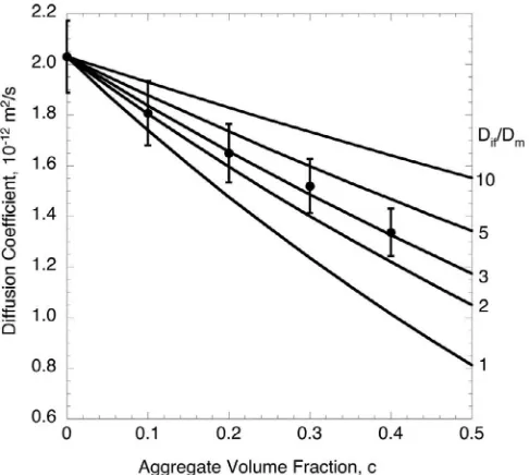
Some data on conductive/diffusive properties of concrete will now be analyzed using the model developed above.Yang and Su (2002)measured the chloride ion diffusivity in a suite of mortar specimens that contained differing volume concentrations of aggregate particles. Two or three samples were prepared and tested at each of five different volume fractions (c) of aggregate. In order to reduce scatter, the average diffusivity at each volume fraction will be used in the analysis, as was done by Yang et al. The diffusivity of the pure cement paste, estimated from the samples havingc=0, was 2.03×10−12_m2_{/s. The diffusivity reduced to}

1.34×10−12_m2_{/s when the inclusion concentration reached 40%. The diffusivities are plotted inFig. 5, as a function of inclusion}

(i.e., aggregate particle) concentration. The error bars indicate the roughly±7% spread of the diffusivities that were measured at each concentration.

The mean inclusion radius, estimated from Table 5 ofYang and Su (2002), is about 0.6 mm, or 600 mm. Although ac-tual inclusion particles are not perfectly spherical, it is known that when inclusions are non-conductive, small deviations from sphericity are of little consequence (Zimmerman, 1989). An ITZ thickness of about 40 mm will be assumed, which is in the range of values commonly reported or estimated (Shane et al., 2000), which tend to lie between 15 and 50 mm. If Eq.(19)is used to model the diffusivity profile, rather than Eq.(5), the 1:15 ratio of interphase thickness to inclusion radius

Fig. 5. Chloride ion diffusivity of a set of mortar specimens containing various volume concentrations of non-diffusive aggregate particles. Data are fromYang and Su (2002), with each data point representing the average of the diffusivities measured for three specimens having that same concentration. The interphase has a power-law parameter ofβ=10. The model predictions are made from Eqs.(14)–(16),(20), using different values of the diffusivity at the interface between the mortar and the inclusions.

is roughly consistent with a power-law exponent of

β

=10. The normalized diffusivity curves predicted from Eqs.(15), (16), (21), for five different values of the parameterDif/Dm, are shown inFig. 5.

All of the measured diffusivities lie above the lowest curve, labeled asD_if/Dm=1, which corresponds to predictions of the Maxwell model for a material with no interphase zone,i.e., Deff/Dm=(1−c)/(1 + 0.5c). This curve also coincides with the Hashin–

Shtrikman upper bound for a two-phase material consisting of pure cement paste and non-conductive inclusions. The fact that the measured diffusivities lie above the H–Supperbound immediately suggests the presence of a highly diffusive interphase zone. The valueDif/Dm=3 provides a good fit to the data, indicating a local diffusivity at the interface with the inclusion that is about three times that of the bulk cement paste.

Yang and Su (2002)obtained an ITZ/bulk diffusivity ratio of 1.76, using an approximate “engineering” approach in which an extra term was added in parallel to the diffusivity, to reflect the effect of an ITZ that was modeled as a thin,locally homogeneous layer. Their value ofDi f=1.76Dmtherefore represents some sort of average diffusivity throughout the ITZ, and so is roughly

consistent with the ratio of 3 obtained in the present analysis. But models such as those used by Yang et al. are not capable of accounting for the fact that the diffusivity varies locally within the interphase region, which implies, for example, that the diffusivity at the interface is much higher than the mean diffusivity of the ITZ.

7. Summary and conclusions

An analytical model was developed for the conductivity (diffusivity, permeability,etc.) of a material that contains a disper-sion of spherical includisper-sions, each surrounded by an inhomogeneous interphase zone in which the conductivity varies radially according to a power law. The Frobenius series method was used to obtain an exact solution for the problem of a single such inclusion in an infinite matrix. Two versions of the solution were developed, one of which is more computationally convenient for interphase zones that are less conductive than the pure matrix, andvice versa. Maxwell’s homogenization method was then used to estimate the effective macroscopic conductivity of the medium.

Some numerical examples were plotted to indicate the general trends predicted by the model. As the interface conductivity varies, the predicted effective conductivity varies between the classical Maxwell prediction for a two-phase material containing non-conductive inclusions, and the prediction for a material containing superconductive inclusions.

References

Arfken, G. B., & Weber, H. J. (2012).Mathematical methods for physicists(7th ed.). San Diego: Academic Press.

Benveniste, Y. (2012). Two models of three-dimensional thin interphases with variable conductivity and their fulfillment of the reciprocal theorem.Journal of the Mechanics and Physics of Solids, 60, 1740–1752.

Benveniste, Y., & Miloh, T. (1999). Neutral inhomogeneities in conduction phenomena.Journal of the Mechanics and Physics of Solids, 36, 762–781. Caré, S., & Hervé, E. (2004). Application of an-phase model to the diffusion coefficient of chloride in mortar.Transport in Porous Media, 56, 119–135.

Cheng, H., & Torquato, S. (1997). Effective conductivity of dispersions of spheres with a superconducting interface.Proceedings of the Royal Society of London Series A, 453, 1331–1344.

Coddington, E. A. (1961).An introduction to ordinary differential equations. Englewood Cliffs, N.J.: Prentice-Hall.

Crumbie, A. K. (1994).Characterisation of the microstructure of concrete(Ph.D. thesis). London, UK: Imperial College.

Drzal, L. T., Rich, M. J., Koenig, M. F., & Lloyd, P. F. (1983). Adhesion of graphite fibers to epoxy matrices: II. The effect of fiber finish.Journal of Adhesion, 16, 133–152. Hashin, Z. (1983). Analysis of composite materials: A survey.Journal of Applied Mechanics, 50, 481–505.

Hashin, Z. (2001). Thin interphase/imperfect interface in conduction.Journal of Applied Physics, 89, 2261–2267.

Hervé, E. (2002). Thermal and thermoelastic behaviour of multiply coated inclusion-reinforced composites.International Journal of Solids and Structures, 39, 1041–1058.

Hinch, E. J. (1991).Perturbation methods. New York: Cambridge University Press.

Kanaun, S. K. (1984). On singular models of a thin inclusion in a homogeneous elastic medium.Prikl. Matem. Mekhan., 48, 50–58.

Kanaun, S. K., & Kudryavtseva, L. T. (1986). Spherically layered inclusions in a homogeneous elastic medium.Prikl. Matem. Mekhan., 50, 633–643. Lutz, M. P., & Ferrari, M. (1993). Compression of a sphere with radially varying elastic moduli.Composites Engineering, 3, 873–884.

Lutz, M. P., Monteiro, P. J. M., & Zimmerman, R. W. (1997). Inhomogeneous interfacial transition zone model for the bulk modulus of mortar.Cement and Concrete Research, 27, 1113–1122.

Lutz, M. P., & Zimmerman, R. W. (1996). Effect of the interphase zone on the bulk modulus of a particulate composite.Journal of Applied Mechanics, 63, 855–861. Lutz, M. P., & Zimmerman, R. W. (2005). Effect of an inhomogeneous interphase zone on the bulk modulus and conductivity of a particulate composite.

Interna-tional Journal of Solids and Structures, 42, 429–437.

Markov, K. Z. (2000). Elementary micromechanics of heterogeneous media. In K. Markov, & L. Preziosi (Eds.),Heterogeneous media: Micromechanics, modeling, methods and simulations(pp. 1–162). Boston: Birkhauser.

Maxwell, J. C. (1873).A treatise on electricity and magnetism. Oxford: Clarendon Press.

Mogilevskaya, S. G., Stolarski, H. K., & Crouch, S. L. (2012). On Maxwell’s concept of equivalent inhomogeneity: When do the interactions matter?Journal of the Mechanics and Physics of Solids, 60, 391–417.

Sevostianov, I. (2014). On the shape of effective inclusion in the Maxwell homogenization scheme for anisotropic elastic composites.Mechanics of Materials, 75, 45–59.

Sevostianov, I., & Kachanov, M. (2007). Effect of interphase layers on the overall elastic and conductive properties of matrix composites: Applications to nanosize inclusion.International Journal of Solids and Structures, 44, 1304–1315.

Sevostianov, I., Levin, V., & Radi, E. (2015). Effective properties of linear viscoelastic microcracked materials: Application of Maxwell homogenization scheme.

Mechanics of Materials, 84, 28–43.

Shane, J. D., Mason, T. O., Jennings, H. M., Garboczi, E. J., & Bentz, D. P. (2000). Effect of the interfacial transition zone on the conductivity of Portland cement mortars.Journal of the American Ceramic Society, 83, 1137–1144.

Shen, L., & Li, J. (2005). Homogenization of a fibre/sphere with an inhomogeneous interphase for the effective elastic moduli of composites.Proceedings of the Royal Society of London Series A, 461, 1475–1504.

Theocaris, P. S. (1992). The elastic moduli of the mesophase as defined by diffusion processes.Journal of Reinforced Plastics and Composites, 11, 537–551. Xie, Y. T., Corr, D. J., Jin, F., Zhou, H., & Shah, S. P. (2015). Experimental study of the interfacial transition zone (ITZ) of model rock-filled concrete (RFC).Cement and

Concrete Composites, 55, 223–231.

Yang, C. C., & Su, J. K. (2002). Approximate migration coefficient of interfacial transition zone and the effect of aggregate content on the migration coefficient of mortar.Cement and Concrete Research, 32, 1559–1565.

Zimmerman, R. W. (1989). Thermal conductivity of fluid-saturated rocks.Journal of Petroleum Science and Engineering, 3, 219–227.