AUTOMATIC POWERLINE SCENE CLASSIFICATION AND RECONSTRUCTION
USING AIRBORNE LIDAR DATA
Gunho Sohn*,Yoonseok Jwa, Heungsik Brian Kim
GeoICT Lab, Geomatics Engineering Program, Earth and Space Science and Engineering Department, York University, Toronto, Canada - (gsohn, yjwa, hskim,)@yorku.ca
KEY WORDS: Power Line Risk Management, 3D Modeling, Classification, Segmentation, Airborne LiDAR Data
ABSTRACT:
This study aims to introduce new methods for classifying key features (power lines, pylons, and buildings) comprising utility corridor scene using airborne LiDAR data and modelling power lines in 3D object space. The proposed approach starts from PL scene segmentation using Markov Random Field (MRF), which emphasizes on the roles of spatial context of linear and planar features as in a graphical model. The MRF classifier identifies power line features from linear features extracted from given corridor scenes. The non-power line objects are then investigated in a planar space to sub-classify them into building and non-building class. Based on the classification results, precise localization of individual pylons is conducted through investigating a prior knowledge of contextual relations between power line and pylon. Once the pylon localization is accomplished, a power line span is identified, within which power lines are modelled with catenary curve models in 3D. Once a local catenary curve model is established, this initial model progressively extends to capture entire power line points by adopting model hypothesis and verification. The model parameters are adjusted using a stochastic non-linear square method for producing 3D power line models. An evaluation of the proposed approach is performed over an urban PL corridor area that includes a complex PL scene.
1. INTRODUCTION
An efficient and reliable monitoring of potential threats on power line (PL) networks has become critical as electricity demands dramatically increase in today’s life and industry. A PL network is comprised of conductors, insulators, pylons and other associated structures (spacer, dead lines, switch boxes and etc.). The PL networks are often exposed to potential threats, which are mainly caused by encroaching vegetation, structural changes between “as-built” and “as-is” condition and violating clearance between conductors and assets (Franken, 2003; Sohn and Ituen, 2010). To mitigate these risks, a timely and accurate monitoring of PL features and their spatial relations is urgently required. Traditionally, this utility monitoring task has been achieved primarily relying on on-site manual inspection, which is expensive, time-consuming and often shows inaccurate results. To overcome this limitation, airborne LiDAR has been lately getting popularity as a primary information source to detect PL risks. This emerging data acquisition tool provides an opportunity to classify a utility corridor scene more reliably and thus generate accurate 3D models of PL features due to LiDAR’s ability of highly dense and multiple-echo data acquisition. Associating 3D models of PL features with PL risk monitoring tasks would provide several advantages against conventional manual on-site investigation. First, vegetation is dynamically growing towards PL conductors. It is critical to timely identify and predict danger trees to PL structures. If PLs are modelled with high accuracy (a design accuracy of conductor’s sag position is in the order of 15 cm), these models can be added to a regular monitoring of vegetation clearance. For instance, having accurate PL models can determine clearance areas that could be jeopardized by a vegetation encroachment by simulating a conductor blowout that shows its maximum designed sag and swing position as well as the potential growth rate of vegetation. Second, PL models provide benefits to investigate violations of ground clearance. The sag positions of conductors vary with atmospheric conditions (i.e., ambient temperature, snow/ice load, solar radiation and so on) and electric current flow. If a conductor’s temperature increases,
its sag position drops down to the underlying terrain surface, which causes a mechanical failure of the PL system. To mitigate this risk, PL models can be used for conducting thermal re-rating, which involves calculating its temperature, sag position, and tension under a variety of conditions. Third, as a PL structure wears out over time, its management should be carried out in a timely manner to prevent electric failures. For example, as the corrosion of a pylon accelerates quickly after 30 years, older pylons should be inspected regularly within a shorter time period to identify their inelastic deformations (Smith and Hall, 2011). PL models are used as for detecting structural anomalies of PL structures by examining movements in their positions over time. This paper aims to introduce several new methods in classifying PL scenes, pylon localization and 3D PL modelling.
2. PREVIOUS RESEARCH
Despite its significance and demands to develop new methods, there have been not much research efforts that are directly related to PL scene classification and modelling using airborne LiDAR data. Baillard and Maître (1999) introduced Markov Random Field (MRF) classifier to identify ground, vegetation and buildings from optical point clouds. Recently, Kim and Sohn (2010) described a PL scene classifier using Random Forests where a number of features were extracted in a point-wise manner. The same authors (2011) proposed a Multiple Classifier System (MCS) for classifying PL scenes, which fuses two Random Forests (RF) classifiers respectively trained from two independent feature set (point- and object-based features). Calberg et al. (2009) developed a series of binary classifiers, each of which can filter out a particular class from unlabelled LiDAR data remained by a previous classifier. Pylons can be considered as a vertical object (tree trunk, traffic light lamp post, etc). Although no research publication can be found in pylon detection, there has been increasing interests in detecting vertical objects from ground-based ranging imagery. Lehtomäki et al. (2010) recognized street posts based on clustering of isolated points on horizontal cross-section. Kim and Medioni (2011) utilized a liner property measured by analyzing the
covariance matrix of local points. Detecting pylons play a key role to isolate individual spans. The previous works in the PL detection and modeling can be divided into two categories: 3D point-based approaches (Melzer and Briese 2004, Clode and Rottensteiner 2005, McLaughlin 2006, Vale and Gomes-Mota 2007, Jwa et al. 2009) and 2D image-based approaches (Yan et al. 2007, Li et al. 2010). Existing methods have demonstrated its successful performance, but in limited environments. For instance, McLaughlin (2006), Yan et al. (2007), and Jwa et al. (2009) reported approximately 72%, 90%, and 94% complete PL extraction rate in the point clouds and imagery data, respectively. The modeling errors mainly depend on scene complexity and data characteristics. In 2D images, the reported approaches might be sensitive to varying image gradients between PLs (voltage types) and their background (i.e., rural versus urban areas). In 3D point clouds, an irregularity in data distribution due to systematic/random errors and occlusions leads to failures in PL modeling completion.
3. METHODOLOGY
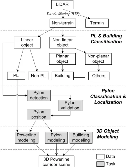
Figure 1 schematically illustrates the overall workflow of the subsequent processes in which three major components, PL scene segmentation, pylon localization, and 3D object modeling are proposed in this study.
Figure 1. Overall workflow for 3D reconstruction of objects including PL, pylon, and building in the PL corridor scene.
3.1 PL and building classification
Figure 2(a) presents a typical PL scene in urban cities which contains ground, PL, electric pylon, building, vegetation, vehicle, other low objects. The first classification step aims to label laser point clouds into linear and non-linear features, which are subsequently classified into PL and building objects. A key aspect in our classification is to consider PL as a set of linear features, while building as a set of planar features. Moreover, contextual properties such as linearity or
co-planarity amongst them are also considered as key properties to distinguish each others. We adopt Markov Random Field (MRF) to characterize unique (data attachment) and contextual properties of those features. In a graph model G = (V, E) comprised of vertices (V) and edges (E), the potential energy of a vertex is calculated by
(1)
where is the data energy term to describe the vertex and is the contextual energy term to describe the consistency with neighbouring vertex linked as a edge. and are the weighting parameters of and respectively (Baillard and Maître, 1999). When over all the vertices is minimized, the iterative optimization process is finished.
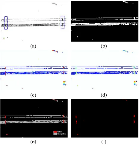
3.1.1 PL classification: A first step of the classification is to label point clouds into two groups: {linear, non-linear}. PL and pylon belong to linear features. LiDAR space is decomposed of a number of voxels (1.5m×1.5m×1.5m). Using all points within each voxel, linear candidate points are extracted, mainly using HT-like voting scheme which was proposed by Jwa et al. (2009) (Figure 2(b)). The linear candidate points are then converted into line segments by 3D line fitting based on RANdom SAmple Consensus (RANSAC) (Figure 2(c)). A graph model is generated on the basis of the line segments (i.e., vertices, V) and the connections between them (i.e., edges, E). Only locally connected edges are remained in the graph, i.e., if the distance between a pair of vertices comprising an edge is larger than a specified threshold (1.5m), the edge is discarded. To discriminate PL from others (mostly pylon), we investigate three data terms (height, line slope, and in-out cylinder) and one contextual term (line parallelism) in MRF. The weights of the terms are tuned by trial and error (0.25, 0.25, 0.2, and 0.3). Each of the energy terms has different potential functions depending on the states (i.e., PL or non-PL) of current vertex or neighbouring vertices. The potential energy functions are manually designed according to following bases.
height: PL is overhead, but part of pylon close to ground has
low height.
line slope: PL is horizontal, while pylon is vertical except horizontal cross-arms.
in-out cylinder: is a ratio of point counts in two coaxial (inner of 0.15m radius and outer of 1m) cylinders created from a line segment. PL hardly has points in the space between inner and outer cylinder.
line parallelism: a single PL is generally parallel to others, but pylon shows random distribution.
Our classification problem is to find an optimal state of each line segment minimizing a global energy computed from the potential functions (Figure 2(d)). The state of the line segment having the highest energy is iteratively switched until the global energy converges. The member points of PL line segments are finally labelled into PL (Figure 2(h)).
3.1.2 Building classification: for each voxel, a plane segment is produced using the remaining points (non-linear) after PL classification. RANSAC is employed to find the best plane approximation (Figure 2(e)). We create locally connected graph consisting of vertices (plane segments) and edges (links of pairs of plane segments) as performed in Section 3.1.1. Two data terms (height and plane normal) and one contextual term (co-planarity) are examined for the separation of building and vegetation which are dominant among the non-PL points.
plane normal: is a deviation from the horizontal. Building roofs are mostly flat or gently sloped.
co-planarity: building has smooth planes, while vegetation
leads to randomly distributed planes.
We used 0.6 and 0.4 as the weights of plane normal and
co-planarity. Figure 2(f) depicts the segments classified into
building. Their member points are assigned as building (Figure 2(h)).
(a) (b)
(c) (d)
(e) (f)
(g) (h)
Figure 2. PL scene classification; (a) optical image, (b) linear feature extraction (red), (c) line segments, (d) PL (blue) vs. PL (black), (e) plane segments, (f) building (blue) vs. non-building (black), (g) ground truth, and (h) PL scene classification result.
3.2 Pylon localization
The pylon localization aims to identify linear segments associated with pylons and validate them by investigating contextual relations amongst extracted pylon regions. For instance, if two true pylon regions are connected each other, we should observe PLs between them and the orientation of the line connecting them equal to PL’s directions. We utilize these properties to progressively eliminate false pylon regions. This idea is implemented in a 2D graph analysis.
3.2.1 Pylon detection: the line segments (Figure 3(a)) extracted in section 3.1.1 are converted into a binary image (Figure 3(b)). Each pixel (1m×1m) possesses line segments passing through the pixel. 2D lines in the pylon pixels are mostly perpendicular to ones in PL pixels as shown in figure 3(a). Based on the line orientation comparison, we investigate two cues to identify pylon:
maximum orientation variation (MOV): is a maximum
variation of orientations analyzed from all pairs of lines in a pixel. It is approximately 90 degrees for pylon, while 0 degree for PL (Figure 3(c) is a normalized image from [0, 90] to [0, 1]).
orientation parallelism (OP): is a mean difference between
the orientation of lines in current pixel and ones in neighbouring pixels. This feature is robust against PL lines having incorrect orientation thanks to smoothness effect. This feature shows similar distribution as maximum
orientation variation (Figure 3(d)).
We employ Random Forests (RF) for the binary classification (pylon vs. non-pylon). RF combines a number of decision trees which are generated by learning different training sets (Breiman, 2001). Based on the two cues (MOV and OP), RF classifier is trained. Figure 3(e) presents RF classification results. Pylon segments classified could be split into two or more segments. To obtain connected pylon regions, morphology filters (dilation and erosion) are applied. Figure 3(f) shows a final pylon detection result.
(a) (b)
(c) (d)
(e) (f)
Figure 3. Pylon segmentation; (a) line segments (blue boxes: pylons), (b) binary image from (a), (c) maximum orientation variation [0,1], (d) orientation parallelism [0,1], (e) pylon classification (RF), and (f) pylon segments.
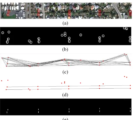
3.2.2 Pylon validation: The pylon detection might produce false positive errors, which need to be pruned. There are ten pylons in our study area as shown in figure 4(a), however our pylon detection method over-detected them (Figure 4(b)). The pylon validation is designed for eliminating non-pylon segment (NPS), while keeping pylon segment (PS) by examining their contextual properties. First, we make all possible connections (edges) among all segments if the edge length is less than a
given value (Figure 4(c)). Then, we identify P edges (connections of PS-PS) and NP edges (PS-NPS or NPS-PS or NPS-NPS). Denote that an edge linking two actual pylons which do not lie on a same PL is considered as NP edge. Let an edge connecting two segments (si and sj) be eij. For the cut of
NP edges, three criteria are found:
F1: , where Ai and Aj are PL pixel
count in regions extended from respective si and sj to the
other segment. The size of the region depends on segment size.
F2: , where and are orientations of
si and sj. is orientation of eij.
F3: , where is the mean orientation of PL pixels between si and sj.
Using three criteria, each edge is scored by the scoring functions (f) that measures its likelihood as P edge. The parameters in the functions were empirically driven. P edge could have very high score over all three criteria, while NP edge would have at least one low score because it does not satisfy all of the criteria. Thus, our edge cutting relies on selecting the lowest score out of three as a representative likelihood (g in Eq. (2)) for each edge.
(2)
The edges are discarded or left based on the likelihood (Figure 4(d)). In this study, we assign an edge whose likelihood is less than 0.5 to NP edge. Finally, the segments corresponding to P edges are labelled into pylon (Figure 4(e)).
(a)
(b)
(c)
(d)
(e)
Figure 4. Pylon validation procedure; (a) true pylon position, (b) detected pylon segments, (c) possible segment connections (edges), (d) remained P-P edges, and (f) pylon detection final result.
3.3 3D PL modeling
This section introduces a new method for automatic 3D PL reconstruction, called Piecewise Model Growing (PMG), suggested by Jwa and Sohn (2012). The algorithm starts from PL primitives extracted in the previous section. We define the 3D PL model using two different geometric form, a two-dimensional line, , of the normal form in X-Y plane and catenary curve, C(a,b,c), of the hyperbolic cosine form in X-Z plane as:
(3) (4)
where are the angle of line’s normal vector and X-axis and the distance between the line and the origin respectively; a
and b are parameters for translation of the origin; c is a scaling factor denoted as the ratio between the tension and the weight of the hanging flexible wire per unit of length; X, Y and Z are the coordinates of the points in 3D space.
The PMG approach estimates the new model parameter vector
w( ) by capturing new PL candidate points along an previous PL model M(wi), and then the new model M(w) is used
as an initial model again for the further progressive propagation. Therefore, M(wi) plays a prominent role as a guild line for
successively gathering PL points neighboured around PL primitive. However, there are two factors that hinder the progressive PL model propagation. First, the point density of neighbouring search space to the current local PL model is not predictable due to the effects of occlusions, shadows, vegetation contacts and system errors. This causes difficulties to achieve accurate model propagation, that is, less and irregular distribution of observations affects results of parameter estimation which might guide the propagation in a wrong direction. The other factor that should be considered to achieve successive model propagation is the hyperbolic nature of the PL catenary curve. To overcome the limitation, we propose incorporating a hypothesis-testing approach into the piecewise model propagation.
3.3.1 PL model hypothesis generation and optimal selection: given PL points D, let Mi denote a PL model in the i-th
piecewise model growing and its model parameter vector wi.
From Mi( ) as a null hypothesis, a sequence of m alternative
models Mi ={Mi( ), Mi ), …, Mi( )}is hypothesized by explicitly changing the given catenary curve’s sag position, b, in Eq. (4) along in Eq. (3). Where, the set of different values of sag position is bj = {b+dbj, j=0,1,…, m | dbj=
}. Since D is used for estimating the parameters of all hypotheses, the estimation process with respect to the variation of bj cannot produce different hypotheses based on the simple
least squares adjustment. To address this problem, we adopted the least squares estimation with stochastic constraints which is a well-understood theory used to consider parameters with weights in a linear function as an additional observation equation (Cothren, 2005). In this case, adjusted parameters in each hypothesis should conform to the overall
geometric deformation caused by . To do this, we modify the normal catenary curve equation by adding two additional parameters (a1,c1) into Eq. (4), which is defined as:
(5)
Consequently, an optimal PL model Mi( ) is selected by using
the hypothesis verification process that measures residuals between Mi( ) and D, and selects a hypothesis satisfying the
best goodness-of-fit criteria as the optimal model in the current propagation step, Mi( )= [D- ]T
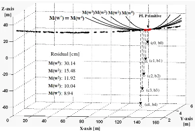
]. Figure 5 illustrates an example for selecting an optimal PL model in the given data domain.
(c0, b0)
(c1, b1)
(c2, b2)
(c3, b3)
(c4, b4)
Y-axis [m] X-axis [m]
Z-axis
[m] PL Primitive
Residual [cm]
: 30.14 : 15.48 : 11.92 : 10.04 : 8.94
Figure 5. Possible alternative hypotheses from M(w0) to M(w4) determined by moving the sag position from b0 to b4 at the current PL primitive (red color) and the selection of the optimal power line model (M(w4) = M(w*)) with the minimum residual.
3.3.2 Piecewise PL model growing: The PMG is subsequently accomplished by generating multiple hypothetical models and selecting an optimal PL model giving the best fit result. This process continues unless Mi( ) is selected as the optimal
model, Mi( ). If is equal to , the propagation
based on the hypothesis-testing is terminated, and then the PL model grows by directly capturing PL points based on Mi( )
without the hypothetic validation. As a result, all optimal PL models generating during the PMG which results in a full PL model are comprised of a set of k and (n-k) different optimal PL models for two steps’ propagation schemes, M = {Mi | i=1,…k,…, n} as shown in Figure 6.
(a) (d)
(b) (e)
(c) (f)
Figure 6. Optimal PL model generation (black coloured line) and its corresponding PL points (red coloured points); (a) initial PL model, (b) and (c) PL models from hypothesis-and-test, (d), (e), and (f) PL models from non-hypothesis-and-test, (f) final PL reconstruction.
3.4 3D Building Modeling
Prismatic building models are extracted from points representing building objects based on the implicit geometric regularization method (Jwa et al., 2008). After building boundary points are traced by using a modified convex-hull
method, noisy boundary vectors are regularized based on Minimum Description Length (MDL) theory.
4. EXPERIMENTAL RESULTS
The urban test area is located in Sacramento, California, USA covers 750m (length) 110m (width). For the data acquisition,
Riegl’s LMS Q560 laser scanner which was attached to a helicopter-borne platform at an altitude of 120 m above ground level was used. The average point density and point distance on PLs is approximately 16 points/m2 and 0.3 m, respectively. Classification was manually conducted by using TerraScan software developed by Terrasolid Ltd to perform quality assessment of the proposed method. As depicted in Figure 7, the test area shows the high-degree PL scene complexity in which there are several voltage types (i.e., 115 kV and 230 kV) and various objects including PLs, pylons, buildings, and vegetation.
(a)
(b)
(c)
(d)
Figure 7. (a) Raw airborne laser scanning data set, (b) PL scene segmentation, (c) Prismatic building reconstruction, and (d) 3D PL structure’s reconstruction: PLs (red colour) and pylons (green colour)
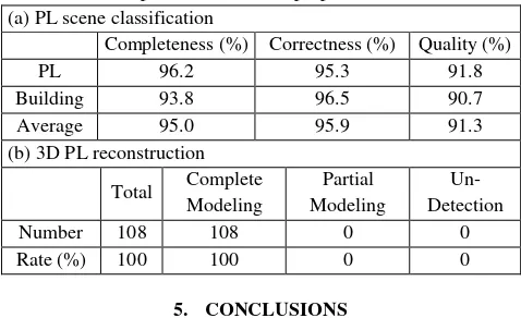
Table 1 shows the overall performance of proposed approach in terms of three criteria (completeness, correctness, and quality) for PL scene classification and modeling completeness for PL reconstruction. The three criteria are formulated by measuring the following factors: TP (True Positive), FN (False Negatives), and FP (False Positive) which are the number of points representing target features found in both the reference and the result, only in the reference, and only in the result, respectively. As a result, the completeness means the detection rate of features of interest. The correctness denotes how well results accurately match the reference. The quality provides the overall performance of results (Rutzinger et al., 2009).
A total number of 49993 and 520074 points were labeled as PL and building in the reference data. Comparing to the reference, TP, FP, and FN are counted as 48085, 2379, and 1908 for PLs, and 487611, 17721, and 32463 for buildings, respectively. This leads to 95%, 95.9%, and 91.3% average success rate for two objects in the term of completeness, correctness, and quality. In the PL modeling, 108 PLs are visually counted in the test site
and all of them are reconstructed completely with less than 6 cm in 3D PL modeling accuracy. In addition, a total of ten pylons (i.e., five for 115 kV and five for 230 kV) and 127 buildings are visually identified in the test area. Pylons and buildings are detected and modelled with 100% (10) and 92% (116) success rate, respectively.
Table 1. Overall performance of the proposed method (a) PL scene classification
Completeness (%) Correctness (%) Quality (%)
PL 96.2 95.3 91.8
An overall approach for classifying and modeling major objects in the urban PL corridor area is presented in this study. The proposed algorithm works well with high success rates in 91.3% overall quality of PL scene classification, 100% and 92% PL and building modeling. These results demonstrate that the proposed method is very promising in practical use. Future research direction is to apply the proposed method to a long PL corridor area containing high-degree PL scene complexity (i.e., diversified voltage types and features in the urban and rural area) for evaluating intensively its performance.
ACKNOWLEDGEMENTS
This research was supported by a grant “Spatiotemporal Risk Management of Power-line Networks” funded by OCE (Ontario Centre for Excellence), NSERC (Natural Sciences and Engineering Research Council) of Canada and GeoDigital International Inc.
REFERENCE
Baillard, C. and Maître, H., 1999, 3D Reconstruction of Urban Scenes from Aerial Stereo Imagery: A Focusing Strategy,
Computer Vision and Image Understanding, 76(3), pp. 244–258.
Breiman, L., 2001, Random Forests, Machine Learning, 45(1), pp. 5-32.
Carlberg, M., Gao, P., Chen, G. and Zakhor, A., 2009 Classifying urban landscape in aerial lidar using 3d shape analysis.In IEEE International Conference on Image Processing.
Clode, S., Rottensteiner, F., 2005. Classification of trees and power lines from medium resolution airborne laserscanner data in urban environments. Proceedings of APRS Workshop on
Digital Image Computing, Brisbane, Australia, CD-ROM.
Franken, P., 2003. Transmission line monitoring through airborne modeling, Fugro-Inpark B.V., Netherlands.
Jwa, Y., Sohn, G., 2012. A piece-wise catenary curve model growing for 3D power line reconstruction. Photogrammetric
Engineering & Remote Sensing (Accepted).
Jwa, Y., Sohn, G., Kim, H., B., 2009. Automatic 3D Powerline Reconstruction Using Airborne LIDAR Data, IAPRS, 38(Part3), pp. 105-110.
Jwa, Y., Sohn, G., Tao, V., Cho, W., 2008. An implicit geometric regularization of 3D building shape using airborne LiDAR data. IAPRS, 37(Part B3a), pp. 69-76.
Kim, E., and G. Medioni, 2011. Urban Scene Understanding from aerial and ground LIDAR data, Machine Vision and
Applications (MVA), 22(4), pp. 691 – 703.
Kim, H.B. and Sohn, G., 2010. 3D Classification of Power-line Scene from Airborne Laser Scanning Data. Photogrammetric Computer Vision (PCV) 2010, ISPRS Commission III Symposium, September 1-3, Paris, France.
Kim, H. B. and Sohn, G., 2011. Random Forests based Multiple Classifier System for Powerline Scene Classification. ISPRS
Laserscanning 2011, Vol. 38.
Lehtomäki, M., A. Jaakkola, J. Hyyppä, J., A. Kukko, and H. Kaartinen, 2010. Detection of Vertical Pole-Like Objects in a Road Environment Using Vehicle-Based Laser Scanning Data.
Remote Sensing, 2(3), pp. 641-664.
Li, Z., Liu, Y., Walker, R., Hayward, R., Zhang, J., 2010. Toward automatic power line detection for a UAV surveillance system using pulse coupled neural filter and an improved hough transform. Machine Vision and Applications, 21(5), pp. 677-686.
McLaughlin, R. A., 2006. Extracting transmission lines from airborne lidar data. IEEE Geoscience and Remote Sensing
Letters, 3(2), pp. 222-226.
Melzer, T., Briese, C., 2004. Extraction and modeling of power lines from ALS point clouds. Proceedings of 28th Workshop of
the Austrian Association for Pattern Recognition (OAGM),
Hagenberg, Austria, pp. 47-54.
Rutzinger, M., Rottensteiner, F., Pfeifer, N., 2009. A comparison of evaluation techniques for building extraction from airborne laser scanning. IEEE Selected Topics in Applied
Earth Observations and Remote Sensing, 2(1), pp. 11-20.
Smith, J., Hall, F., 2011. A proactive approach to tower maintenance, Transmission & Distribution World, 63(2), pp. 56F-56I.
Sohn, G. and Dowman, I. J., 2002. Terrain surface reconstruction by the use of tetrahedron model with the MDL criterion. In: Proceedings the Photogrammetric Computer
Vision, Vol. 34, pp.336-344.
Sohn, G., Ituen, I., 2010. The Way Forward: Advances in maintaining Right-Of-Way of transmission lines. GEOMATICA, 64(40), pp. 451-462.
Vale, A., Gomes-Mota, J., 2007. Lidar data segmentation for track clearance anomaly detection on over-head power lines.
Proceedings of IFAC Workshop, Yzmir, Turkey, pp. 17-19.
Yan, G., Li C., Zhou, G., Zhang, W., Li, X., 2007. Automatic extraction of power lines from aerial images. IEEE Geoscience
and Remote Sensing Letters, 4(3), pp. 387-391.