Tools for Verifying Classical
and Quantum Superintegrability
Ernest G. KALNINS †, Jonathan M. KRESS ‡ and Willard MILLER Jr.§
† Department of Mathematics, University of Waikato, Hamilton, New Zealand
E-mail: [email protected]
URL: http://www.math.waikato.ac.nz
‡ School of Mathematics, The University of New South Wales, Sydney NSW 2052, Australia
E-mail: [email protected]
URL: http://web.maths.unsw.edu.au/∼jonathan/
§ School of Mathematics, University of Minnesota, Minneapolis, Minnesota,55455, USA
E-mail: [email protected]
URL: http://www.ima.umn.edu/∼miller/
Received June 04, 2010, in final form August 06, 2010; Published online August 18, 2010
doi:10.3842/SIGMA.2010.066
Abstract. Recently many new classes of integrable systems in ndimensions occurring in classical and quantum mechanics have been shown to admit a functionally independent set of 2n−1 symmetries polynomial in the canonical momenta, so that they are in fact su-perintegrable. These newly discovered systems are all separable in some coordinate system and, typically, they depend on one or more parameters in such a way that the system is superintegrable exactly when some of the parameters are rational numbers. Most of the con-structions to date are forn= 2 but cases wheren >2 are multiplying rapidly. In this article we organize a large class of such systems, many new, and emphasize the underlying mecha-nisms which enable this phenomena to occur and to prove superintegrability. In addition to proofs of classical superintegrability we show that the 2D caged anisotropic oscillator and a St¨ackel transformed version on the 2-sheet hyperboloid are quantum superintegrable for all rational relative frequencies, and that a deformed 2D Kepler–Coulomb system is quantum superintegrable for all rational values of a parameterkin the potential.
Key words: superintegrability; hidden algebras; quadratic algebras
2010 Mathematics Subject Classification: 20C99; 20C35; 22E70
1
Introduction
We define an n-dimensional classical superintegrable system to be an integrable Hamiltonian system that not only possessesnmutually Poisson – commuting constants of the motion, but in addition, the Hamiltonian Poisson-commutes with 2n−1 functions on the phase space that are globally defined and polynomial in the momenta. Similarly, we define a quantum superintegrable system to be a quantum Hamiltonian which is one of a set ofnindependent mutually commuting differential operators, and that commutes with a set of 2n−1 independent differential opera-tors of finite order. We restrict to classical systems of the form H = Pn
i,j=1gijpipj +V and
corresponding quantum systemsH = ∆n+ ˜V. These systems, including the classical Kepler and
quantum symmetries as differential operators. Systems of 2nd order have been well studied and there is now a structure and classification theory [3, 4, 5, 6, 7, 8]. For 3rd and higher order superintegrable systems much less is known. In particular there have been relatively few examples and there is almost no structure theory. However, within the last three years there has been a dramatic increase in discovery of new families of possible higher order superintegrable classical and quantum systems [9,10,11,12,13,14,15,16]. The authors and collaborators have developed methods for verifying superintegrability of these proposed systems, [17, 18, 19, 20]. In the cited papers the emphasis was on particular systems of special importance and recent interest. Here, however, the emphasis is on the methods themselves.
In Section 2 we review a method for constructing classical constants of the motion of all orders for n-dimensional Hamiltonians that admit a separation of variables in some orthogonal coordinate system. Then we apply it to the case n= 2 to show how to derive superintegrable systems for all values of a rational parameterkin the potential. Many of our examples are new. In Section3we review our method for establishing a canonical form for quantum symmetry oper-ators of all orders for 2-dimensional Schr¨odinger operators such that the Schr¨odinger eigenvalue equation admits a separation of variables in some orthogonal coordinate system. Then we apply this method to establish the quantum superintegrability of the caged anisotropic oscillator for all frequencies that are rationally related, and for a St¨ackel transformed version of this system on the 2-sheet hyperboloid. We give a second proof for the caged oscillator in all dimensionsnthat relies on recurrence relations for associated Laguerre polynomials. We also apply the canonical equations to establish the quantum superintegrability of a deformed Kepler–Coulomb system for all rational values of a parameterk in the potential.
1.1 The construction tool for classical systems
There are far more verified superintegrable Hamiltonian systems in classical mechanics than was the case 3 years ago. The principal method for constructing and verifying these new systems requires that the system is already integrable, in particular, that it admits a separation of variables in some coordinate system. For a Hamiltonian system in 2n-dimensional phase space the separation gives us n second order constants of the motion in involution. In this paper we first review a general procedure, essentially the construction of action angle variables, which yields an additional n−1 constants, such that the set of 2n−1 is functionally independent. This is of little interest unless it is possible to extract nnew constants of the motion that are polynomial in the momenta, so that the system is superintegrable. We will show how this can be done in many cases. We start first with the construction of action angle variables for Hamiltonian systems in ndimensions, and later specialize to the case n= 2 to verify superintegrability.
Consider a classical system in n variables on a complex Riemannian manifold that admits separation of variables in orthogonal separable coordinates x1, . . . , xn. Then there is ann×n
St¨ackel matrix
S = (Sij(xi))
such that Φ = detS6= 0 and the Hamiltonian is
H=L1 =
n
X
i=1
T1i p2i +vi(xi)
=
n
X
i=1
T1i p2i +V(x1, . . . , xn),
where V =Pn
i=1T1i vi(xi),T is the matrix inverse toS:
n
X
j=1
TijSjk = n
X
j=1
and δik is the Kronecker delta. Here, we must require Πni=1T1i 6= 0. We define the quadratic
constants of the motion Lk,k= 1, . . . , n by
Lk = n
X
i=1
Tki p2i +vi
, k= 1, . . . , n,
or
p2i +vi = n
X
j=1
SijLj, 1≤i≤n. (2)
As is well known,
{Lj,Lk}= 0, 1≤j, k≤n.
Here,
{A(x,p),B(x,p)}=
n
X
i=1
(∂iA ∂piB −∂piA ∂iB).
Furthermore, by differentiating identity (1) with respect toxh we obtain
∂hTiℓ=− n
X
j=1
TihShj′ Tjℓ, 1≤h, i, ℓ≤n,
where S′
hj =∂hShj.
Now we define nonzero functionsMkj(xj, pj,L1, . . . ,Ln) on the manifold by the requirement
{Mkj,Lℓ}=TℓjSjk, 1≤k, j, ℓ≤n.
It is straightforward to check that these conditions are equivalent to the differential equations
2pj∂jMkj+ −v′j+ n
X
q=1 Sjq′ Lq
!
∂pjMkj =Sjk, 1≤j, k≤n.
We can use the equalities (2) to consider Mkj either as a function ofxj alone, so that dxdjMkj = Sjk/2pj or as a function of pj alone. In this paper we will take the former point of view.
Now define functions
˜
Lq = n
X
j=1
Mqj, 1≤q≤n.
Then we have
{L˜q,Lℓ}= n
X
j=1
TℓjSjq =δℓq. (3)
This shows that the 2n−1 functions
H=L1,L2, . . . ,Ln,L˜2, . . . ,L˜n,
Now let’s consider how this construction works in n = 2 dimensions. By replacing each separable coordinate by a suitable function of itself and the constants of the motion by suitable linear combinations of themselves, if necessary, e.g. [21], we can always assume that the St¨ackel matrix and its inverse are of the form
S =
where fj is a function of the variable xj alone. The constants of the motion L1 = H and L2
are given to us via variable separation. We want to compute a new constant of the motion ˜L2
functionally independent of L1,L2. Setting M21=M, M22=−N, we see that
The treatment of subgroup separable superintegrable systems in n dimensions, [18], is also a special case of the above construction. Suppose the St¨ackel matrix takes the form
S =
which leads exactly to the construction found in [18].
1.2 Application of the construction for n = 2
As we have seen, forn= 2 and separable coordinatesu1=x,u2 =y we have
We will present strategies for determining functions f1, f2, v1, v1 such that there exists a 3rd constant of the motion, polynomial in the momenta. The constant of the motion ˜L2 =M−N
constructed by solving equations (4) is usually not a polynomial in the momenta, hence not directly useful in verifying superintegrability. We describe a procedure for obtaining a polynomial constant from M−N, based on the observation that the integrals
can often be expressed in terms of multiples of the inverse hyperbolic sine or cosine (or the ordinary inverse sine or cosine), and the hyperbolic sine and cosine satisfy addition formulas. Thus we will search for functions fj, vj such that M and N possess this property. There is a larger class of prototypes for this construction, namely the second order superintegrable systems. These have already been classified for 2-dimensional constant curvature spaces [4] and, due to the fact that every superintegrable system on a Riemannian or pseudo-Riemannian space in two dimensions is St¨ackel equivalent to a constant curvature superintegrable system [22,23], this list includes all cases. We will typically start our construction with one of these second order systems and add parameters to get a family of higher order superintegrable systems.
A basic observation is that to get inverse trig functions for the integralsM,N we can choose the potential functions f(z),v(z) from the list
Z1(z) =Az2+Bz+C, Z2(z) =
A+Bsinpz
cos2py ,
Z3(z) = A cos2pz +
B
sin2pz, Z4(z) =Ae
2ipz+Beipz,
Z5(z) =Az2+ B
z2, Z6(z) = A
z + B z2,
sometimes restricting the parameters to special cases. Many of these cases actually occur in the lists [4] so we are guaranteed that it will be possible to construct at least one second order polynomial constant of the motion from such a selection. However, some of the cases lead only to higher order constants.
Cartesian type systems
For simplicity, we begin with Cartesian coordinates in flat space. The systems of this type are related to oscillators and are associated with functionsZj forj = 1,5,6. We give two examples.
[E1]. For our first construction we give yet another verification that the extended caged har-monic oscillator is classically superintegrable. We modify the second order superintegrable system [E1], [4], by looking at the potential
V =ω12x2+ω22y2+ β
x2 + γ y2,
with L2 = p2x+ω21x2 + xβ2. (For ω1 = ω2 this is just [E1].) It corresponds to the choice of
a function of the formZ5 for each of v1,v2. Evaluating the integrals, we obtain the solutions
M(x, px) = i
4ω1A, sinhA= i(2ω2
1x2− L2)
p
L2
2−4ω12β ,
N(y, py) = − i
4ω2B, sinhB= i(2ω2
2y2− H+L2)
p
(H − L2)2−4ω22γ ,
to within arbitrary additive constants. We choose these constants so thatM,N are proportional to inverse hyperbolic sines. Then, due to the formula cosh2u−sinh2u = 1, we can use the identities (2) to compute coshA and coshB:
coshA= p2ω1xpx
L22−4ω21β
, coshB= p 2ω2ypy (H − L2)2−4ω22γ
.
Now suppose that ω1/ω2 = k is rational, i.e. k = pq where p, q are relatively prime integers.
Then ω1 =pω,ω2 =qω and
are both constants of the motion. Each of these will lead to a polynomial constant of the motion. Indeed, we can use the relations
(coshx±sinhx)n= coshnx±sinhnx,
cosh(x+y) = coshxcoshy+ sinhxsinhy,
sinh(x+y) = coshxsinhy+ sinhxcoshy,
coshnx=
[n/2]
X
j=0
n
2j
sinh2jx coshn−2jx,
sinhnx= sinhx
[(n=1)/2]
X
j=1
n
2j−1
sinh2j−2xcoshn−2j−1x.
recursively to express each constant as a polynomial in coshA, sinhA, coshB, sinhB. Then, writing each constant as a single fraction with denominator of the form
((H − L2)2−4ω22γ)n1/2(L22−4ω12β)n2/2
we see that the numerator is a polynomial constant of the motion. Note that, by construction, both sinh(−4ipqω[M−N]) and cosh(−4ipqω[M−N]) will have nonzero Poisson brackets withL2,
hence they are each functionally independent of H,L2. Since each of our polynomial constants
of the motion differs from these by a factor that is a function ofH, L2 alone, each polynomial
constant of the motion is also functionally independent of H, L2. Similar remarks apply to all
of our examples.
[E2]. There are several proofs of superintegrability for this system, but we add another. Here, we make the choicev1=Z1,v2=Z5, corresponding to the second order superintegrable system [E2]
in [4]. The potential is
V =ω12x2+ω22y2+αx+ β
y2,
whereL2 =p2x+ω21x2+αxand the system is second order superintegrable for the caseω1=ω1.
Applying our method we obtain
M(x, px) = i
2ω1A
, sinhA= i(ω
2 1x+α)
p
4ω21L2+α2
, coshA= p 2ω1px 4ω12L2+α2
,
N(y, py) = i
4ω2B
, sinhB= i(2ω
2
2y2− H+L2)
p
(H − L2)2−4ω22β
, coshB= p 2ω2ypy (H − L2)2−4ω22β
.
Thus if ω1/2ω2 is rational we obtain a constant of the motion which is polynomial in the
momenta.
Polar type systems
Next we look at flat space systems that separate in polar coordinates. The Hamiltonian is of the form
H=p2r+ 1
r2 p 2
θ+f(r) +g(θ)
=e−2R p2R+pθ2+v1(R) +v2(θ)
,
Cases for which the whole process works can now be evaluated. Possible choices of f and g are
In each case if p is rational there is an extra constant of the motion that is polynomial in the canonical momenta.
[E1]. Case (1) is system [E1] fork= 1. For general k this is the TTW system [12], which we have shown to be supperintegrable for krational.
Case (2). This case is not quadratic superintegrable, but as shown in [19] it is superintegrable for all rational k.
[E8]. For our next example we take Case (3) wherez=x+iy:
for arbitraryk. (Ifk= 2 this is the nondegenerate superintegrable system [E8] listed in [4].) In polar coordinates, with variablesr =eR and z=eR+iθ. Then we have
This system is superintegrable for all rational k.
[E17]. TakingCase (4) we have, forz=x+iy:
(For k= 1 this is the superintegrable system [E17] in [4].) Then we have
H =e−2R p2R+p2θ+αeR+βe−2ikθ+γe−ikθ
, (5)
−L2 =p2θ+βe−2ikθ+γe−ikθ, H=e−2R p2R− L2+αeR
.
Applying our procedure we find the functions
N(θ, pθ) =
This demonstrates superintegrability for all rational k.
[E16]. Case (5)corresponds to [E16] fork= 1, and our method shows that it is superintegrable for all rational k.
Spherical type systems
These are systems that separate in spherical type coordinates on the complex 2-sphere. The Hamiltonian is of the form
H= cosh2ψ p2ψ+p2ϕ+v1(ϕ) +v2(ψ)
,
x=ϕ, y=ψ, f1= 0, f2= 1 cosh2ψ.
Embedded in complex Euclidean 3-space with Cartesian coordinates, such 2-sphere systems can be written in the form
H =J12+J22+J32+V(s),
where
J3 =s1ps2 −s2ps1, J1 =s2ps3−s3ps2, J2=s3ps1 −s1ps3, s 2
1+s22+s33 = 1.
[S9]. Here, we have the casev1(ϕ) =Z3 and v2(ψ) is a special case ofZ3.
V = α
s2 1
+ β
s2 2
+ γ
s2 3 .
It is convenient to choose spherical coordinates
s1= cosϕ
sinhψ, s2 = sinϕcoshψ, s3= tanhψ.
In terms of these coordinates the Hamiltonian has the form
H= cosh2ψ
p2ψ+p2ϕ+ α cos2ϕ+
β
sin2ϕ+ γ
sinh2ψ
,
L2 =p2ϕ+ α
cos2ϕ+ β
sin2ϕ, H= cosh 2ψ
p2ψ+L2+ γ
sinh2ψ
,
system [S9] in [4]. We extend this Hamiltonian via the replacement ϕ→kϕ and proceed with our method. Thus
H= cosh2ψ
p2ψ+p2ϕ+ α cos2kϕ+
β
sin2kϕ+ γ
sinh2ψ
,
L2 =p2ϕ+ α
cos2kϕ+ β
sin2kϕ
with Hexpressed as above. The functions that determine the extra constant are
M(ϕ, pϕ) = i
4k√L2A ,
sinhA= ip(L2cos(2kϕ)−α+β) (L2−α−β)2−4αβ
, coshA= p sin(2kϕ)pϕ (L2−α−β)2−4αβ
,
N(ψ, pψ) = i
4√L2B ,
sinhB= pi(L2cosh(2ψ) +γ− H) (H+L2−γ)2+ 4L2γ
, coshB= p isinh(2ψ)pψ (H+L2−γ)2+ 4L2γ
.
[S7]. This system corresponds tov1(φ) = Z2 and v2(ψ) a variant of Z3. The system is second
Choosing the coordinates ψ andϕ we find
H= cosh2ψ
We make the transformation ϕ→kϕand obtain
H= cosh2ψ
with Has before. The functions that determine the extra constants are
M(ϕ, pϕ) = √1
Thus this system is superintegrable for all rational k.
[S4]. Herev1(ϕ) =Z4 and v2(ψ) is a variant of Z2. This is another system on the sphere that
is second order superintegrable and separates in polar coordinates:
V = α
In terms of angular coordinates ψ,ϕthe Hamiltonian is
H= cosh2ψ
After the substitutionϕ→kϕ we have
L2 =p2ϕ+αe2ikϕ+γikϕ, H= cosh2ψ
The functions that determine the extra constants are
M(ϕ, pϕ) = i
[S2]. Herev1(ϕ) =Z4 and v2(ψ) is a variant ofZ3:
V = α
s2 3
+ β
(s1−is2)2
+γ(s1+is2) (s1−is2)3 .
which is is second order superintegrable. After the substitution ϕ→kϕwe obtain the system
H= cosh2ψ
p2ψ+p2ϕ+ α
sinh2ψ+βe
2ikϕ+γe4ikϕ
, (6)
L2 =p2ϕ+βe2ikϕ+γe4ikϕ, H= cosh2ψ
p2ψ+L2+ α
sinh2ψ
.
Applying our procedure we find
M(ϕ, pϕ) = i
4√L2kA
, sinhA= (2L2e
−ikϕ−β)
p
4L2γ−β2
, coshA= 2
√ L2pϕ
p
4L2γ−β2 e−ikϕ,
N(ψ, pψ) = i
4√L2B ,
sinhB= pi(L2cosh(2ψ)−α+H) (L2−α− H)2−4αH
, coshB=
√
L2sinh(2ψ)pψ
p
(L2−α− H)2−4αH .
Thus the system is superintegrable for all rational k.
1.3 Horospherical systems
In terms of horospherical coordinates on the complex sphere we can construct the Hamiltonian
H=y2 p2x+p2y+ω12x2+ω22y2+α+βx
.
If ω1/ω2 is rational then this system is superintegrable. However, there is no need to go into
much detail for the construction because a St¨ackel transform, essentially multiplication by 1/y2, takes this system to the flat space system generalizing [E2] and with the same symmetry algebra.
There is a second Hamiltonian which separates on the complex 2 sphere
H =y2p2x+p2y + α
x2 +β+ω 2
1x2+ω22y2
.
It is superintegrable for ω1/ω2 rational, as follows from the St¨ackel transform 1/y2 from the sphere to flat space. If ω1 = ω2 then we obtain the system [S2]. We note that each of the
potentials associated with horospherical coordinates can quite generally be written in terms of s1,s2,s3 coordinates using the relations
y= −i
s1−is2
, x= −s3
s1−is2
, s21+s22+s23 = 1.
1.4 Generic systems
These are systems of the form
H= 1
Zj(x)−Zk(y)
p2x−p2y + ˆZj(x)−Zˆk(y)
,
wherej,kcan independently take the values 2, 3, 4 and Zj, ˆZj depend on distinct parameters. Superintegrability is possible because of the integrals
Z
dx
√
C+Be2ikx+Ae4ikx =
1
2k√Carcsin
2Ce−2ikx+B
√
4AC−B2
Z
dx
q
A+Bsinkx cos2kx +C
=− 1
k√C arcsin
−2Csinkx+B
√
4C2+ 4CA+B2
,
Z
dx
q
A cos2
kx+ B sin2
kx +C
=− 1
2k√Carcsin
Ccos 2kx+A−B
p
(A+B+C)2−4AB
!
.
Consider an example of this last type of system:
H= 1
A′e2ikx+B′e4ikx−a′e2iqy−b′e4iqy p 2
x−p2y+Ae2ikx+Be4ikx−ae2iqy−be4iqy
.
The equation H=E admits a separation constant
p2x+ (A−EA′)e2ikx+ (B−EB′)e4ikx =p2y + (a−Ea′)e2iqy+ (b−Eb′)e4iqy=L.
As a consequence of this we can find functions M(x, px) andN(y, py) where
M(x, px) =
1
4k√Larcsin
2 ˆAe−2ikx+ ˆB
p
4LAˆ−Bˆ2
!
,
where ˆA=A−EA′, ˆB =B−EB′ and
N(y, py) = 1
4p√Larcsin
2ˆae−2iqy+ ˆb
p
4Lˆa−ˆb2
!
,
where ˆa = a−Ea′, ˆb = b−Eb′. We see that if q
k is rational then we can generate an extra
constant which is polynomial in the momenta.
The superintegrable systems that have involved the rational functions Z1, Z5 and Z6 work
because of the integrals
Z dx
√
Ax2+Bx+C =
1
√
Aarcsinh
2Ax+C
√
4AB−C2
and
Z
dx
x√Ax2+Bx+C =−
1
√
B arcsinh
2B+Ax x√A2−4BC
.
2
Quantum superintegrability
2.1 The canonical form for a symmetry operator
We give a brief review of the construction of the canonical form for a symmetry operator [19]. Consider a Schr¨odinger equation on a 2D real or complex Riemannian manifold with Laplace– Beltrami operator ∆2 and potential V:
HΨ≡(∆2+V)Ψ =EΨ
that also admits an orthogonal separation of variables. If {u1, u2} is the orthogonal separable coordinate system the corresponding Schr¨odinger operator has the form
H =L1 = ∆2+V(u1, u2) = 1 f1(u1) +f2(u2)
∂u21 +∂ 2
u2 +v1(u1) +v2(u2)
and, due to the separability, there is the second-order symmetry operator
L2 = f2(u2)
f1(u1) +f2(u2)
∂u21+v1(u1)
−f f1(u1)
1(u1) +f2(u2)
∂u22+v2(u2)
,
i.e., [L2, H] = 0,and the operator identities
f1(u1)H+L2=∂u21 +v1(u1), f2(u2)H−L2 =∂ 2
u2 +v2(u2).
We look for a partial differential operator ˜L(H, L2, u1, u2) that satisfies
[H,L˜] = 0.
We require that the symmetry operator take the standard form
˜
L=X
j,k
Aj,k(u1, u2)∂u1u2 +B j,k(u
1, u2)∂u1+C j,k(u
1, u2)∂u2+D j,k(u
1, u2)
HjLk2. (8)
We have shown that we can write
˜
L(H, L2, u1, u2) =A(u1, u2, H, L2)∂12+B(u1, u2, H, L2)∂1
+C(u1, u2, H, L2)∂2+D(u1, u2, H, L2), (9)
and consider ˜L as an at most second-order order differential operator inu1,u2 that is analytic
in the parameters H, L2. Then the conditions for a symmetry can be written in the compact form
Au1u1 +Au2u2+ 2Bu2 + 2Cu1 = 0, (10) Bu1u1+Bu2u2−2Au2v2+ 2Du1−Av
′
2+ (2Au2f2+Af ′
2)H−2Au2L2= 0, (11) Cu1u1+Cu2u2 −2Au1v1+ 2Du2 −Av
′
1+ (2Au1f1+Af ′
1)H+ 2Au1L2 = 0, (12) Du1u1+Du2u2 −2Bu1v1−2Cu2v2−Bv
′ 1−Cv2′
+ (2Bu1f1+ 2Cu2f2+Bf ′
1+Cf2′)H+ (2Bu1−2Cu2)L2 = 0. (13)
We can further simplify this system by noting that there are two functionsF(u1, u2, H, L2), G(u1, u2, H, L2) such that (10) is satisfied by
A=F, B =−1
2∂2F−∂1G, C=− 1
2∂1F+∂2G. (14)
Then the integrability condition for (11), (12) is (with the shorthand ∂jF = Fj, ∂jℓF = Fjℓ,
etc., for F and G),
2G1222+
1
2F2222+ 2F22(v2−f2H+L2) + 3F2(v
′
2−f2′H) +F(v′′2 −f2′′H)
−2G1112+
1
2F1111+ 2F11(v1−f1H−L2) + 3F1(v
′
1−f1′H) +F(v1′′−f1′′H), (15)
and equation (13) becomes 1
2F1112+ 2F12(v1−f1H) +F1(v
′
2−f2′H) +
1
2G1111+ 2G11(v1−f1H−L2)
+G1(v1′ −f1′H) =−
1
2F1222−2F12(v2−f2H)−F2(v
′
1−f1′H) +
1 2G2222
Here, any solution of (15), (16) with A, B, C not identically 0 corresponds to a symmetry operator that does not commute with L2, hence is algebraically independent of the
symmet-riesH,L2. (Informally, this follows from the construction and uniqueness of the canonical form of a symmetry operator. The operators ˜L=g(H, L2) algebraically dependent on H and L2 are
exactly those such that A=B =C= 0, D=g(H, L2). A formal proof is technical.) Note also
that solutions of the canonical equations, withH,L2 treated as parameters, must be interpreted in the form (8) withH and L2 on the right, to get the explicit symmetry operators.
2.2 The caged anisotropic oscillator
In [19] we used the canonical form for symmetry operators to demonstrate the quantum superin-tegrability of the TTW system [12,13] for all rationalk, as well as a system on the 2-hyperboloid of two sheets [19]. Here we give another illustration of this construction by applying it to the 2D caged oscillator [11]. Forp=q This is the second order superintegrable system [E1] on complex Euclidean space, as listed in [4]. Here,
HΨ = (∂11+∂22+V(u1, u2))Ψ, (17)
where
V(u1, u2) =ω2 p2u21+q2u22
+α1
u21 + α2 u22,
in Cartesian coordinates. We take p,q to be relatively prime positive integers. Thus
f1 = 1, f2 = 0, v1 =ω2p2u21+ α1
u21, v2 =ω 2q2u2
2+ α2 u22.
The 2nd order symmetry operator is
L2 =− ∂22+v2(u2)
,
and we have the operator identities
∂12=−(v1(u1) +H+L2), ∂22 =−v2(u2) +L2.
Based on the results of [18] for the classical case, we postulate expansions of F,G in finite series
F =X
a,b
Aa,bEa,b(u1, u2), G=
X
a,b
Ba,bEa,b(u1, u2), Ea,b(u1, u2) =ua1ub2. (18)
The sum is taken over terms of the forma =a0+m, b= b0+n, and c = 0,1, where m, n
are integers. The point (a0, b0) could in principle be any point inR2,
Taking coefficients with respect to the basis (18) in each of equation (15) and (16) gives recurrence relations for these coefficients. The shifts in the indices ofA andB are integers and so we can view this as an equation on a two-dimensional lattice with integer spacings. While the shifts in the indices are of integer size, we haven’t required that the indices themselves be integers, although they will turn out to be so in our solution. The 2 recurrence relations are of a similar complexity, but rather than write them out separately, we will combine them into a matrix recurrence relation by defining
Ca,b=
Aa,b Ba,b
· · · · · · • · · · · · · · · • · · · · · · • · · · · · · • · • · • · · · · ◦ · • · • · · · · • · · · · · · · ·
Figure 1. The template. Points contributing to the recurrence relation are marked with large dots (•,◦). The large dot on the bottom center corresponds to the position (a−1, b+ 1), the large dot at the top corresponds to the position (a+ 4, b) and◦corresponds to position (0,0).
We write the 2 recurrence relations in matrix form as
0=Ma,bCa,b+Ma−1,b+1Ca−1,b+1+Ma,b+2Ca,b+2+Ma,b+4Ca,b+4
+Ma+1,b−1Ca+1,b−1+Ma+1,b+1Ca+1,b+1+Ma+1,b+3Ca+1,b+3+Ma+2,bCa+2,b
+Ma+3,b+1Ca+3,b+1+Ma+4,bCa+4,b,
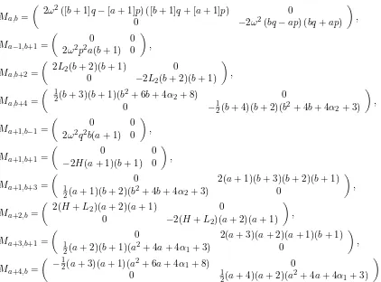
where eachMi,j is a 2×2 matrix given below.
Ma,b=
2ω2([b+ 1]q−[a+ 1]p) ([b+ 1]q+ [a+ 1]p) 0
0 −2ω2(bq−ap) (bq+ap)
,
Ma−1,b+1 =
0 0
2ω2p2a(b+ 1) 0
,
Ma,b+2=
2L2(b+ 2)(b+ 1) 0
0 −2L2(b+ 2)(b+ 1)
,
Ma,b+4=
1
2(b+ 3)(b+ 1)(b2+ 6b+ 4α2+ 8) 0
0 −12(b+ 4)(b+ 2)(b2+ 4b+ 4α2+ 3)
,
Ma+1,b−1 =
0 0
2ω2q2b(a+ 1) 0
,
Ma+1,b+1 =
0 0
−2H(a+ 1)(b+ 1) 0
,
Ma+1,b+3 =
0 2(a+ 1)(b+ 3)(b+ 2)(b+ 1)
1
2(a+ 1)(b+ 2)(b2+ 4b+ 4α2+ 3) 0
,
Ma+2,b=
2(H+L2)(a+ 2)(a+ 1) 0
0 −2(H+L2)(a+ 2)(a+ 1)
,
Ma+3,b+1 =
0 2(a+ 3)(a+ 2)(a+ 1)(b+ 1)
1
2(a+ 2)(b+ 1)(a2+ 4a+ 4α1+ 3) 0
,
Ma+4,b=
−12(a+ 3)(a+ 1)(a2+ 6a+ 4α1+ 8) 0
0 12(a+ 4)(a+ 2)(a2+ 4a+ 4α1+ 3)
.
points with the opposite parity. A second simplification results from the fact that the recurrence matricesMa+m,b+nare of two distinct types. Eitherm,nare both even, in which caseMa+m,b+n
is diagonal, or m, n are both odd, in which case the diagonal elements of Ma+m,b+n are zero.
Another simplification follows from the observation that it is only the ratiop/q=r that matters in our construction. We want to demonstrate that the caged anisotropic oscillator is operator superintegrable for any rational r. The construction of any symmetry operator independent of H and L2 will suffice. By writing ω=ω′/2,p′ = 2p,q′ = 2q inH, we see that, without loss
of generality, we can always assume that p,q are both even positive integers with a single 2 as their only common factor.
If for a particular choice ofp, q we can find a solution of the recurrence relations with only a finite number of nonzero vectors Ca,b then there will be a minimal lattice rectangle with
vertical sides and horizontal top and bottom that encloses the corresponding lattice points. The top row a0 of the rectangle will be the highest row in which nonzero vectors Ca0,b occur.
The bottom row a1 will be the lowest row in which nonzero vectors Ca1,b occur. Similarly,
the minimal rectangle will have right column b0 and left column b1. Now slide the template
horizontally across the top row such that only the lowest point on the template lies in the top row. The recurrence gives (a0 + 1)bAa0,b = 0 for all columns b. Based on examples for the
classical system, we expect to find solutions for the quantum system such that a0 ≥ 0 and b ≥ 0. Thus we require Aa0,b = 0 along the top of the minimal lattice rectangle, so that all
vectors in the top row take the form
Ca0,b=
0
Ba0,b
.
Now we move the template such that the recurrence Ma,b, second row from the bottom and on
the left, lies on top of the lattice point (a0, b0). This leads to the requirement (b0q−a0p)(b0q+ a0p)Ba0,b0 = 0. Again, based on hints from specific examples, we postulate Ba0,b0 6= 0, a0 =q, b0 =p. Since we can assume thatp,qare even, this means that all odd lattice points correspond to zero vectors. Next we slide the template vertically down column b0 such that only the left
hand point on the template lies in column b0. The recurrence gives (b0−1)aAa,b0 = 0 for all
rows a. Sinceb0 is even, we postulate that
Ca,b0 =
0
Ba,b0
for all lattice points in column b0.
Note that the recurrence relations preserve the following structure which we will require:
1. There is only the zero vector at any lattice point (a, b) witha+b odd.
2. If the row and column are both even then Ca,b=
0
Ba,b
.
3. If the row and column are both odd then Ca,b=
Aa,b
0
.
This does not mean that all solutions have this form, only that we are searching for at least one such solution.
To finish determining the size of the minimum lattice rectangle we slide the template vertically downward such that only the right hand point on the template lies in columnb1. The recurrence gives (b1−1)(b1−3)A(a, b1) = 0,b1(b1−2)Ba,b1 = 0 for all rowsa. There are several possible
solutions that are in accordance with our assumptions, the most conservative of which isb1 = 0.
In the following we assume only thatBa0,b0 6= 0, the structure laid out above, and the necessary
a vector at a lattice point that is not determined by the recurrences we shall assume it to be zero. Our aim is to find one nonzero solution with support in the minimum rectangle, not to classify the multiplicity of all such solutions.
Now we carry out an iterative procedure that calculates the values of Ca,b at points in the
lattice using only other points where the values of Ci,j are already known. We position the
template such that the recurrence Ma,b, second row from the bottom and on the left (of the
template), lies above the lattice point (a0, b),a0 =q, and slide it from right to left along the top
row. The caseb=b0 =p has already been considered. For the remaining cases we have
2ω2p2a0(b+ 1)Aa0−1,b+1= 2ω2(bq−a0p)(bq+a0p)Ba0,b+ 2L2(b+ 2)(b+ 1)Ba0,b+2
+1
2(b+ 4)(b+ 2)(b
2+ 4b+ 4α
2+ 3)Ba0,b+4. (19)
Only even values ofbneed be considered. Now we lower the template one row and again slide it from right to left along the row. The contribution of the lowest point on the template is 0 and we find
2ω2(q[b+ 2]−p[a0])(q[b+ 2] +p[a0])Aa0−1,b+1=−2a0(b+ 4)(b+ 3)(b+ 2)Ba0,b+4
−2L2(b+ 3)(b+ 2)Aa0−1,b+3−
1
2(b+ 4)(b+ 2)(b
2+ 8b+ 11α2+ 8)A
a0−1,b+5, (20)
where we have replaced bby b+ 1 so that again only even values of bneed be considered. For the first step we takeb=p−2. Then equation (19) becomes
2ω2p3qAq−1,p−1=−8ω2q2(p−1)Bq,p−2+ 2L2p(p−1)Bq,p,
and (20) is vacuous in this case, leavingAq−1,p−1 undetermined. Note that several of the terms
lie outside the minimal rectangle. From these two equations we can solve forBq,p−2 in terms of
our givenBq,p,Aq−1,p. Now we march across both rows from right to left. At each stage our two
equations now allow us to solve uniquely for Aq−1,b+1 and Bq,b in terms of A’s and B’s to the
right (which have already been computed). We continue this until we reachb= 0 and then stop. At this point the top two rows of the minimal rectangle have been determined by our choice of Bq,p and Aq−1,p−1. We repeat this construction for the third and fourth rows down, then the
next two rows down, etc. The recurrence relations grow more complicated as the higher rows of the template give nonzero contributions. However, at each step we have two linear relations
2ω2p2a(b+ 1) −2ω2(bq−ap)(bq+ap) 2ω2(q[b+ 2]−pa)(q[b+ 2] +pa) 0
Aa−1,b+1 Ba,b
=· · · ,
where the right hand side is expressed in terms ofA’s andB’s either above or on the same line but to the right of Aa−1,b+1,Ba,b, hence already determined. Since the determinant of the 2×2
matrix is nonzero over the minimal rectangle, except for the upper right corner and lower left corner, at all but those those two points we can compute Aa−1,b+1, Ba,b uniquely in terms of
quantities already determined. This process stops with rows a= 1,2.
Row a = 0, the bottom row, needs special attention. We position the template such that the recurrence Ma,b lies above the lattice point (0, b), and slide it from right to left along the
bottom row. The bottom point in the template now contributes 0 so at each step we obtain an expression for B0,b in terms of quantities A,B from rows either above row 0 or to the right of
column b in row 0, hence already determined. Thus we can determine the entire bottom row, with the exception of the value at (0,0), the lower left hand corner. When the point Ma,b on
the template is above (0,0) the coefficient of B0,0 vanishes, so the value of B0,0 is irrelevant
constants χ,η. Hence if, for example,χ6= 0 we can require Bq,p =−(η/χ)Aq−1,p−1 and satisfy
this condition while still keeping a nonzero solution. Thus after satisfying this linear condition we still have at least a one parameter family of solutions, along with the arbitrary B0,0 (which is clearly irrelevant since it just adds a constant to the function G). However, we need to check those recurrences where the pointMa,b on the template slides along rowsa=−1,−2,−3,−4 to
verify that these relations are satisfied. We have already utilized the casea=−4, and for cases
a=−3,−2,−1 it is easy to check that the relations are vacuous.
The last issue is the left hand boundary. We have determined all vectors in the minimal rectangle, but we must verify that those recurrences are satisfied where the point Ma,b on the template slides along columns b=−1,−2,−3,−4. However again the recurrences are vacuous.
We conclude that there is a one-parameter (at least) family of solutions to the caged aniso-tropic oscillator recurrence with support in the minimal rectangle. By choosing the arbitrary parameters to be polynomials in H, L2 we get a finite order constant of the motion. Thus the
quantum caged anisotropic oscillator is superintegrable. We note that the canonical operator construction permits easy generation of explicit expressions for the defining operators in a large number of examples. Once the basic rectangle of nonzero solutions is determined it is easy to compute dozens of explicit examples via Maple and simple Gaussian elimination. The generation of explicit examples is easy; the proof that the method works for all orders is more challenging.
Example. Taking p = 6 and q = 4, we find (via Gaussian elimination) a solution of the recurrence with nonzero coefficients
A1,1, A1,3, A1,5, A3,1, A3,3, A3,5,
B0,2, B0,4, B2,0, B2,2, B2,4, B4,0, B4,2, B4,4, B6,0, B6,2, B6,4.
We can take A1,5 =a1 and A3,3 =a2 and then all other coefficients will depend linearly on a1
and a2. Calculating theA,B, C and D from equations (11), (12), (14) we find the coefficient
ofH−1 has a factor of 2a
2+ 9a1 and so we seta1 =ω6 anda2 =−9/2a1 to obtain the symmetry
operator ˜L, (9), where u1,u2 are Cartesian coordinates and
+
Using Maple, we have checked explicitly that the operator ˜L commutes with H. Note that it is of 6th order. Taking the formal adjoint ˜L∗, [19], we see thatS = 1
2( ˜L+ ˜L∗) is a 6th order,
formally self-adjoint symmetry operator.
3
An alternate proof of superintegrability
for the caged quantum oscillator
This second proof is very special for the oscillator and exploits the fact that separation of variables in Cartesian coordinates is allowed Here we write the Hamiltonian in the form
H =∂x2+∂y2−µ21x2−µ22y2+ find the normalized solutions
Xn=e−
where the Lαn(x) are associated Laguerre polynomials [24]. For the corresponding separation constants we obtain
The total energy is −λx−λy =E. Taking µ1=pµand µ2 =qµ wherep and q are integers we
find that the total energy is
E =−2µ(pn+qm+pa1+p+qa2+q).
Therefore, in order thatE remain fixed we can admit values of integersm and nsuch that
pn+qm is a constant. One possibility that suggests itself is that n →n+q,m → m−p. To see that this is achievable via differential operators we need only consider
Ψ =La1
n (z1)Lam2(z2), z1 =µ1x2, z2=µ2y2.
We now note the recurrence formulas for Laguerre polynomials viz.
x d dxL
α
p(x) =pLαp(x)−(p+α)Lαp−1(x) = (p+ 1)Lαp+1(x)−(p+ 1 +α−x)Lαp(x).
Because of the separation equations we can associate p with a differential operator for bothm
and n in the expression for Ψ. We do not change the coefficients of Lαp±1(x). Therefore we can raise or lower the indices m and nin Ψ using differential operators. In particular we can perform the transformation n→n+q,m→m−p and preserve the energy eigenvalue. To see how this works we observe the formulas
D+(µ1, x)Xn= ∂2x−2xµ1∂x−µ1+µ21x2+ 1 4−α21
x2
!
Xn=−4µ1(n+ 1)Xn+1,
D−(µ2, y)Ym= ∂y2+ 2yµ2∂y+µ2+µ22y2+ 1 4 −α22
y2
!
Ym =−4µ2(m+α2)Ym−1.
In particular, if we make the choice µ1 = 2µ, µ2 = µ then the operator D+(2µ, x)D−(µ, y)2
transformsXnYmto−128µ3(n+1)(m+α2)(m−1+α2)Xn+1Ym−2. We see that this preserves the
energy eigenspace. Thus can easily be extended to the case whenµ1=pµandµ2=qµforpandq
integers. A suitable operator isD+(pµ, x)qD−(qµ, y)p. Hence we have constructed a differential
operator that commutes with H! The caged oscillator is quantum superintegrable. This works to prove superintegrability in all dimensions as we need only take coordinates pairwise.
Remark. This second proof of superintegrability, using differential recurrence relations for Laguerre polynomials is much more transparent than the canonical operator proof, and it gen-eralizes immediately to all dimensions. Unfortunately, this oscillator system is very simple and the recurrence relation approach is more difficult to implement for more complicated potentials. Special function recurrence relations have to be worked out. Also, we only verified explicitly the commutivity on an eigenbasis for a bound state.
3.1 A proof of superintegrability for a deformed Kepler–Coulomb system
In [16] there is introduced a new family of Hamiltonians with a deformed Kepler–Coulomb potential dependent on an indexing parameter k which is shown to be related to the TTW oscillator system system via coupling constant metamorphosis. The authors showed that this system is classically superintegrable for all rational k. Here we demonstrate that this system is also quantum superintegrable. The proof follows easily from the canonical equations for the system.
The quantum TTW system isHΨ =EΨ with H given by (7) where
v2 = β
cos2(kθ) + γ
sin2(kθ) =
2(γ+β) sin2(2kθ)+
2(γ−β) cos(2kθ) sin2(2kθ) .
(Setting r = eR we get the usual expression for this system in polar coordinates r, θ.) In our paper [19] we used the canonical form for symmetry operators to establish the superintegrability of this system. Our procedure was, based on the results of [20] for the classical case, to postulate expansions ofF,Gin finite series
F =X
a,b,c
Aa,b,cEa,b,c(R, θ), G=
X
a,b,c
Ba,b,cEa,b,c(R, θ),
Ea,b,0 =e2aRsinb(2kθ), Ea,b,1 =e2aRsinb(2kθ) cos(2kθ).
The sum is taken over terms of the form a=a0+m,b=b0+n, andc= 0,1, where m,n are
integers,a0 is a positive integer andb0 is a negative integer. HereF,Gare the solutions of the
canonical form equations (14), (15), (16) for the TTW system. We succeeded in finding finite series solutions for all rationalk, and this proved superintegrability.
In [16] the authors point out that under the St¨ackel transformation determined by the po-tential U =e2R the TTW system transforms to the equivalent system ˆHΨ =−αΨ, where
ˆ
H = 1
e4R
∂R2 +∂θ2−Eexp(2R) + β cos2(kθ) +
γ
sin2(kθ)
. (22)
Then, settingr =e2R, φ= 2θ, we find the deformed Kepler–Coulomb system.
∂r2+1
r +
1
r2∂ 2 φ−
E
4r +
β
4r2cos2(kφ/2)+
γ
4r2sin2(kφ/2)
Ψ =−α 4Ψ.
From the canonical equations, it is virtually immediate that system (22) is superintegrable. Indeed the only difference between the functions (21) defining the TTW system and the functions defining the St¨ackel transformed system is that f1 and v1 are replaced by f1 = exp(4R) and v1 =−Eexp(2R) (we can set E=H) and the former H is replaced by −α. From this we find
that the only difference between the canonical equations for the TTW system and the canonical equations for the transformed system is that α becomes −Hˆ and H becomes −α. Since our proof of the superintegrability of the TTW system did not depend on the values of H and α, the same argument shows the superintegrability of the transformed system. Also, any solution (i.e., a second commuting operator) for the TTW system gives rise to a corresponding operator for the transformed system by replacing α and H with −Hˆ and−α, respectively.
Example. For the deformed Kepler system with k = 2, we take p = 2 and q = 1 and use Gaussian elimination to find a solution with nonzero coefficients
A−2,1,0, A−1,1,0, B−2,0,0, B−2,0,1, B−1,0,0, B−1,0,1, B0,0,1,
in which A−2,1,0 and A−1,1,0 are two independent parameters. To achieve the lowest order
symmetry and ensure that theA,B,C andDare polynomial in ˆL2 and ˆH, we chooseA−2,1,0 =
32( ˆL2−4) and A−1,1,0 = 0 and find,
A= 32e−4Rsin(4θ) ˆL2−128e−4Rsin(4θ),
B = 8e−4Rcos(4θ) ˆL22+ (8(β−γ)e−4R+ 4Ee−2Rcos(4θ)−8e−4Rcos(4θ)) ˆL2
−96e−4Rcos(4θ)−16Ee−2Rcos(4θ) + 40(γ−β)e−4R+ 4E(β−γ)e−2R, C =−8e−4Rsin(4θ) ˆL22−4 sin(4θ) ˆHLˆ2+ 8(e−4R−Ee−2R) sin(4θ) ˆL2+ 20 sin(4θ) ˆH
D=−32e−4Rcos(4θ)L22−8 cos(4θ) ˆHLˆ2
+ (128e−4Rcos(4θ)−12Ee−2Rcos(4θ) + 16(γ−β)e−4R) ˆL
2+ 24 cos(4θ) ˆH
+ 48(β−γ)e−4R+ 48Ee−2Rcos(4θ)−4E(γ−β)e−2R+ 2E2cos(4θ).
It has been explicitly checked, using Maple, that the fifth order operator obtained from these expressions commutes with ˆH.
3.2 A proof of superintegrability for the caged oscillator on the hyperboloid
Using this same idea we can find a new superintegrable system on the 2-sheet hyperboloid by taking a St¨ackel transformation of the quantum caged oscillator HΨ = EΨ, (17) in Cartesian coordinatesu1,u2 by multiplying with the potentialU = 1/u21. The transformed system is
u21
∂12+∂22+ω2u21(p2u21+q2u22)−Eu21+α2 u21 u2 2
Ψ =−α1Ψ.
We embed this system as the upper sheets0 >0 of the 2-sheet hyperboloids20−s21−s22 = 1 in 3-dimensional Minkowski space with Minkowski metricds2 =−ds20+ds21+ds22, via the coordinate transformation
s0=
1 +u21+u22
2u1
, s1 =
1−u21−u22
2u1
, s2 = u2 u1
, u1>0.
Then the potential for the transformed system is
˜
V = α2
s2 2 −
E
(s0+s1)2 +
ω2(p2−q2)
(s0+s1)4 +
ω2q2(s 0−s1)
(s0+s1)3 . (23)
This is an extension of the complex sphere system [S2], distinct from the system (6) that we proved classically superintegrable. It is an easy consequence of the results of [17] that the classical version of system (23) is also superintegrable for all rationally related p, q. However, quantum superintegrability isn’t obvious. However, from the results of Section2.2it is virtually immediate that this new system is quantum superintegrable for all relatively prime positive integers p, q. This follows from writing down the canonical equations (15), (16), first for the caged oscillator where
f1 = 1, f2 = 0, v1 =ω2p2u21+ α1
u21, v2 =ω 2q2u2
2+ α2 u22,
and then for the St¨ackel transformed system where
f1 =
1
u21, f2 = 0, v1 =ω 2p2u2
1−E, v2=ω2q2u22+ α2 u22.
The equations are identical except for the switches α1 → −E, H → −α1. Thus our proof of quantum superintegrability for the caged oscillator carries over to show that the system on the hyperboloid is also quantum superintegrable.
4
Discussion
calculations. Although our primary emphasis in this paper was to develop tools for verifying classical and quantum superintegrabity at all orders, we have presented many new results. The classical Eucidean systems [E8], [E17] and most of the examples of superintegrability for spaces with non-zero scalar curvature are new. We have explored the limits of the construction of classical superintegrable systems via the methods of Section 1.1 for the case n = 2. Further use of this method will require looking at n >2, where new types of behavior occur, such as appearance of superintegrable systems that are not conformally flat. We also developed the use of the canonical form for a symmetry operator to prove quantum superintegrability. We applied the method to then= 2 caged anisotropic oscillator to give the first proof of quantum superintegrability for all rational k. We used the St¨ackel transform together with the canonical equations to give the first proofs of quantum superintegrability for all rationalkof a 2D deformed Kepler–Coulomb system, and of the caged anisotropic oscillator on the 2-hyperboloid. Then we introduced a new approach to proving quantum superintegrability via recurrence relations obeyed by the energy eigenfunctions of a quantum system, and gave an alternate proof of the superintegrabilty for all rationalkof the caged anisotropic oscillator. This proof clearly extends to all n. The recurrences for the caged oscillator are particularly simple, but the method we presented shows great promise for broader application. Clearly, we are just at the beginning of the process of discovery and classification of higher order superintegrable systems in all dimensions n >2.
References
[1] Tempesta P., Winternitz P., Harnad J., Miller W. Jr., Pogosyan G. (Editors), Superintegrability in classical and quantum systems (Montr´eal, 2002),CRM Proceedings and Lecture Notes, Vol. 37, American Mathema-tical Society, Providence, RI, 2004.
[2] Eastwood M., Miller W. Jr. (Editors), Symmetries and overdetermined systems of partial differential equa-tions, Summer Program (Minneapolis, 2006), The IMA Volumes in Mathematics and its Applications, Vol. 144, Springer, New York, 2008.
[3] Kalnins E.G., Kress J.M., Miller W. Jr., Second-order superintegrable systems in conformally flat spaces. V. Two- and three-dimensional quantum systems,J. Math. Phys.47(2006), 093501, 25 pages.
[4] Kalnins E.G., Kress J.M., Pogosyan G.S., Miller W. Jr., Completeness of superintegrability in two-dimensional constant curvature spaces,J. Phys. A: Math Gen.34(2001), 4705–4720,math-ph/0102006.
[5] Daskaloyannis C., Ypsilantis K., Unified treatment and classification of superintegrable systems with inte-grals quadratic in momenta on a two dimensional manifold,J. Math. Phys. 47(2006), 042904, 38 pages,
math-ph/0412055.
[6] Kalnins E.G., Kress J.M., Miller W. Jr., Nondegenerate three-dimensional complex Euclidean superinte-grable systems and algebraic varieties,J. Math. Phys.48(2007), 113518, 26 pages,arXiv:0708.3044.
[7] Kalnins E.G., Miller W. Jr., Post S., Wilson polynomials and the generic superintegrable system on the 2-sphere,J. Phys. A: Math. Theor.40(2007), 11525–11538.
[8] Kalnins E.G., Miller W. Jr., Post S., Quantum and classical models for quadratic algebras associated with second order superintegrable systems,SIGMA4(2008), 008, 21 pages,arXiv:0801.2848.
[9] Chanu C., Degiovanni L., Rastelli G., Superintegrable three-body systems on the line, J. Math. Phys. 49
(2008), 112901, 10 pages,arXiv:0802.1353.
[10] Rodriguez M.A., Tempesta P., Winternitz P., Reduction of superintegrable systems: the anisotropic har-monic oscillator,Phys. Rev. E78(2008), 046608, 6 pages,arXiv:0807.1047.
Rodriguez M.A., Tempesta P., Winternitz P., Symmetry reduction and superintegrable Hamiltonian systems,
J. Phys. Conf. Ser.175(2009), 012013, 8 pages,arXiv:0906.3396.
[11] Verrier P.E., Evans N.W., A new superintegrable Hamiltonian,J. Math. Phys.49(2008), 022902, 8 pages,
arXiv:0712.3677.
[13] Tremblay F., Turbiner A., Winternitz P., Periodic orbits for an infinite family of classical superintegrable systems,J. Phys. A: Math. Theor.43(2010), 015202, 14 pages,arXiv:0910.0299.
[14] Quesne C., Superintegrability of the Tremblay–Turbiner–Winternitz quantum Hamiltonians on a plane for oddk,J. Phys. A: Math. Theor.43(2010), 082001, 10 pages,arXiv:0911.4404.
[15] Tremblay F., Winternitz P., Third order superintegrable systems separating in polar coordinates,J. Phys. A: Math. Theor.43(2010), 175206, 17 pages,arXiv:1002.1989.
[16] Post S., Winternitz P., An infinite family of superintegrable deformations of the Coulomb potential,
J. Phys. A: Math. Theor.43(2010), 222001, 11 pages,arXiv:1003.5230.
[17] Kalnins E.G., Miller W. Jr., Post S., Coupling constant metamorphosis andNth-order symmetries in classical
and quantum mechanics,J. Phys. A: Math. Theor.43(2010), 035202, 20 pages,arXiv:0908.4393.
[18] Kalnins E.G., Kress J.M., Miller W. Jr., Families of classical subgroup separable superintegrable systems,
J. Phys. A: Math. Theor.43(2010), 092001, 8 pages,arXiv:0912.3158.
[19] Kalnins E.G., Kress J.M., Miller W. Jr., Superintegrability and higher order integrals for quantum systems,
J. Phys. A: Math. Theor.43(2010), 265205, 21 pages,arXiv:1002.2665.
[20] Kalnins E.G., Miller W. Jr., Pogosyan G.S., Superintegrability and higher order constants for classical and quantum systems,Phys. Atomic Nuclei, to appear,arXiv:0912.2278.
[21] Eisenhart L.P., Separable systems of St¨ackel, Ann. of Math. (2)35(1934), 284–305.
[22] Kalnins E.G., Kress J.M., Miller W. Jr., Second order superintegrable systems in conformally flat spaces. II. The classical two-dimensional St¨ackel transform,J. Math. Phys.46(2005), 053510, 15 pages.
[23] Kalnins E.G., Kress J.M., Miller W. Jr., Post S., Structure theory for second order 2D superintegrable systems with 1-parameter potentials,SIGMA5(2009), 008, 24 pages,arXiv:0901.3081.