BUILDING MONITORING WITH DIFFERENTIAL DSMS
A. Alobeid1, K. Jacobsen1, C. Heipke1, M. Al Rajhi1, 2 1
Institute of Photogrammetry and GeoInformation, Leibniz University Hannover
(alobeid, jacobsen, heipke)@ipi.uni-hannover.de
2
Ministry of Municipal and Rural Affairs (MoMRA), Riyadh, KSA
[email protected]
KEY WORDS: DSM, GeoEye-1, IKONOS, aerial photos, least squares matching, semi global matching
EXECUTIVE SUMMARY:
The monitoring of building activity (erection of new buildings, demolishing buildings and especially the change of building heights) by manual inspection of space and aerial images is time consuming and a source of errors. A detection of building changes based on the comparison of digital surface models (DSMs) is more reliable. For this study DSMs have been generated based on aerial images, an IKONOS and a GeoEye-1 stereo pair taken from 2007 up to 2009. By pixel based matching with dynamic programming, semiglobal matching and least squares matching the visible surface has been determined. Semiglobal matching leads to sharp building shapes, while the area based least squares matching smoothes the height model and has more problems in areas with little or without contrast. As is shown in the investigation building changes and building height changes in the range of one floor can in many cases be determined with all methods, however building shapes are better determined using semiglobal matching.
1. INTRODUTION
For a suburb of Riyadh the change of buildings contained in a large scale database over time shall be determined using aerial and satellite images. The cause for change is manifold: buildings can have been missed during the set up of the database, a new section or floor can have been added, or a new, and possibly illegal, building can have been constructed. In order to detect changes, data must be available at appropriate time intervals. The detection of buildings based on a digital surface model (DSM) is much more reliable than processing of single images. Therefore, significantly better results can be expected from this investigation as compared to single image evaluations.
Aerial images from May 2007, an IKONOS stereo pair from 2008 and a GeoEye-1 stereo pair from 2009 are available in addition to the database. Digital Surface Models (DSMs) have been generated by least squares matching (LSM),
pixel based
matching with dynamic programming (DP) according to
(Birchfield and Tomasi 1998) and semiglobal matching
(SGM) according to (Hirschmüller 2008).
2. DATA SETS AND IMAGE ORIENTATION
2.1 Aerial images 1 : 45 000
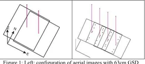
Wide angle aerial photos scanned with 14µm pixel size, corresponding to 63cm ground sampling distance (GSD) – the distance of neighboured projected pixel centres – from May 24th 2007 have been used. The image orientation determined by bundle block adjustment has a sigma naught of 3.6µm and root mean square discrepancies at ground control points (GCP) of 14cm for X, 11cm for Y and 99cm in Z, clearly below the GSD in planimetry, and still acceptable in height. The configuration with 60% end lap can be seen in figure 1 left. As is typical for aerial photos, the scanned images have limited contrast and are
influenced by film grain. With edge analysis (Jacobsen 2008) the effective resolution has been determined with 70cm GSD.
2.2 Aerial images 1 : 5200
Also large scale normal angle photos scanned with 14µm pixel size, corresponding to 7cm GSD from May 25th 2007 are available. The bundle block adjustment resulted in a sigma naught of 2.7µm and mean square discrepancies at GCP of 1.0cm for X, 1.1cm for Y and 4.4cm in Z are also in the sub-pixel accuracy range. The configuration with 60% end lap can be seen in figure 1 right. By edge analysis the effective resolution has been determined with 9cm GSD. Images of both scales show some scanning errors with stripes and sometimes dust.
Figure 1: Left: configuration of aerial images with 63cm GSD Right: configuration of aerial images with 7cm GSD
2.3 IKONOS stereo pair
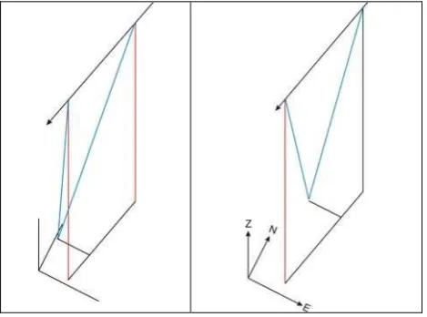
An IKONOS stereo pair from May 24th, 2008 was used with the standard height to base relation h/b=1.75 (b/h=0.57) and a viewing angle of 11° to the West (figure 2 left) with the standard 1m GSD and orientation information available as rational polynomial coefficients (RPC). The RPC are based on the direct sensor orientation determined by a GPS-receiver in the satellite, gyros and star sensors, not supported by GCP. The stereo model orientation with bias corrected RPCs in relation to International Archives of the Photogrammetry, Remote Sensing and Spatial Information Sciences, Volume XXXVIII-4/W19, 2011
22 GCP determined by means of the aerial images has root mean square errors of 0.40m in X, 0.46m in Y and 1.15m in Z. For single image orientation, where the height of the GCP is fixed, the root mean square differences at the GCP are 0.48m for X and 0.60m for Y. The edge analysis did not show a loss of the effective GSD against the nominal GSD.
2.4 GeoEye-1 stereo pair
The used GeoEye-1 stereo pair has been acquired on September 15th 2009 with a height to base relation of h/b=1.5 (b/h=0.66) and a viewing angle of also 11° to the West (figure 2 right). The images have the standard 0.5m GSD. The stereo model orientation with bias corrected RPCs in relation to 22 GCP determined by means of the aerial images has root mean square errors of 0.28m in X, 0.36m in Y and 1.13m in Z. For single image orientation, where the height of the GCP is fixed, the root mean square differences at the GCP are 0.41m for X and 0.48m for Y. Also for the GeoEye-1 images the edge analysis did not show a loss of the effective GSD against the nominal GSD.
Figure 2: imaging constellation. Left: IKONOS, right: GeoEye-1
3. EPIPOLAR IMAGES
Corresponding image points are related to the same object point (figure 3 upper). In the images they are located on epipolar lines – the intersection of the image planes with the plane defined by the projection centres and the object point. Only in aerial images taken in the normal case, with rotations identical to zero and same height of projection centres, the directions of the epipolar lines are identical to the x’-direction, having the same y-coordinate in both images of the stereo model. In the general case the images have different orientations. So the classical image matching with original images searches for corresponding image positions in the x’- and the y’-direction. The search in both directions is time consuming. The original images can be transformed into epipolar images (figure 3 lower), corresponding to normal case images. In such epipolar images the point corresponding to a reference point in the other image has the same y-coordinate, reducing the search from two to one dimension.
Epipolar images are related to one stereo pair; that means if we have three aerial images 1, 2 and 3, we have to generate epipolar images for the images 1 and 2 related to model 1-2 and epipolar images 2 and 3 related to model 2-3. So for image 2 we have one epipolar image for the left model and one for the right
model, both are not identical because the projection centres are usually not located on an exact straight line.
The generation of epipolar images is similar to the generation of orthoimages (except for the need of height information to create orthoimages). The point in the output epipolar image is defined in the output raster and the position of the corresponding point in the original image is computed. The grey values of the position in the original image are used for the epipolar image. As with orthoimages this leads to an interpolation problem because the computed position in the original image usually will not be exactly in a pixel centre. With bilinear interpolation slightly better matching results have been achieved as with nearest neighbourhood interpolation.
Figure 3: Upper: epipolar geometry, lower: epipolar image
The generation of epipolar images is not unequivocal – the projection plane for the epipolar images can be rotated around the image base. The Hannover program EPIPOL for generating epipolar images creates an orientation file for any stereo model including the information about interior and exterior orientation and the geometry of the epipolar transformation. With this file and the corresponding image positions from matching by intersection with program BLINTS, ground coordinates can be computed directly.
In theory epipolar images from satellite line scanner images cannot be computed directly, they require an iterative computation. In practice, this issue can be handled more easily: If images projected to a plane with constant height in the object area, as IKONOS Geo, GeoEye Geo or QuickBird Ortho-ready standard, are available, a simple rotation of the images to the base direction is satisfactory for the generate of epipolar images, since the remaining y-parallaxes are usually below one pixel.
4. IMAGE MATCHING
Corresponding image points are determined by image matching. The classical method of matching is area based – the similarity between a sub-matrix of one image and a sub-matrix of the other is determined. The cross-correlation requires flat object space and images parallel to each other. By least squares matching (LSM) one sub-matrix is transformed to the other using an affine transformation, allowing also inclined terrain and images not being parallel to the ground. Area based matching has the disadvantage that it requires an object plane – this is not the case for buildings with sudden height changes at the facades. As a consequence, in the resulting DSM the sudden height difference appears as low pass filtered. By pixel based matching the building shape can be determined more precisely. Pixel based matching is computationally more demanding, and usually it is based on epipolar images. It is not possible to only match one pixel to another one - it requires additional information, e. g. in the form of a cost function used by pixel based matching with dynamic programming (DP) according to (Birchfield & Tomasi 1998). DP handles one epipolar line independently to the neighbouring one, leading to streaking of the buildings. The streaking can be reduced by filtering with a small matrix perpendicular to the epipolar line. As another pixel based method semiglobal matching (SGM) respects not only the similarity in the epipolar line but also in lines rotated against it (Hirschmüller 2008).
For the building monitoring least squares matching, pixel based matching with dynamic programming and semiglobal matching was used. A detailed explanation of these methods is available in (Alobeid et al., 2010).
5. DSM GENERATION
5.1 Least squares matching
The area based least squares matching generates object points if the similarity between corresponding sub-matrixes exceeds a threshold for the correlation coefficient. This threshold was set to 0.6. For areas show values below this limit gaps exist, which can be filled by interpolation, but such an interpolation is critical as it causes a smoothing of the height model. This is different for the pixel based matching - within the handled epipolar line they are not changing the height if there are no clear changes of the grey values. For building monitoring this has advantages because on top of buildings and sometimes on the ground there is sometimes only little contrast, but in any case at locations with a clear height change grey values do change.
Figure 4: part of corresponding aerial images 63cm GSD
A typical problem of image matching can be seen in figure 4 at the isolated building to the right. In the left image a shadow can be seen on left of building, while the building on the right shows parts of the façade on right hand side. In least squares matching such areas are causing gaps, while the pixel based matching defines it correctly as occlusions.
Figure 5: Aerial image 63cm GSD: left: white = areas with points matched by LSM, right: quality image – grey value of matched points corresponding to correlation coefficient of LSM; grey value = 255 corresponding to r=1.0, grey value 50 to r=0.6
Figure 5 demonstrates the gaps in least squares matching; there are points in areas with low contrast and at areas where left and right image do not correspond at building facades due to different view direction. The limited values of the LSM correlation coefficients for the aerial photos with 63cm GSD can be seen in the quality image in figure 5 as well as in the frequency distribution of the correlation coefficients in figure 7.
Figure 6: Points matched by LSM (white) laid over sub-image, left: aerial photo reduced to 28cm GSD, right: GeoEye-1
Similar to the aerial stereo pairs with 63cm GSD, also the satellite stereo pairs have points not matched by LSM in shadow areas, occlusions and at low contrast areas (figure 6). International Archives of the Photogrammetry, Remote Sensing and Spatial Information Sciences, Volume XXXVIII-4/W19, 2011
Figure 7: frequency distribution of correlation coefficients by LSM
The frequency distribution of the correlation coefficients (figure 7) indicates the image quality. The aerial images with 63cm GSD are disturbed by film grain and have a limited contrast. This is better for the aerial images with 7cm GSD. A ground resolution of 7cm is not required for the determination of buildings, so these images in addition have been linearly reduced by factor 4.0 to 28cm GSD. By averaging 4 x 4 pixels the influence of the film grain disappears, improving also the matching quality to approximately the correlation coefficients as achieved with GeoEye-1 images (figure 7).
Any matching procedure requires approximate information about the result for limiting the search radius. The used Hannover program DPCOR for least squares image matching uses region growing, starting at one or more seed points (known corresponding image points). From the seed point the program goes into 4 neighboured directions for matching the next points. From the improved corresponding positions the program continues to the neighbourhood. If occlusions (e.g. in one image the façade can be seen, but not in the other) are too large or there is no satisfying contrast, the matching of neighboured points fails. If the program cannot continue from all matched points to the neighbourhood, it stops. This is critical for the 7cm GSD images, requiring a high number of seed points, but not for the images reduced by a linear factor 4 to 28cm GSD. LSM is an area based method. It computes the corresponding positions as centre of the used image sub-matrix (template). In the case of a discontinuity within the sub-matrix it only can lead to average height information, smoothing the DSM.
template size 10x10 pixels
template size 6x6 pixels
template size 1x1 pixels
Figure 8: simulated height profiles according to area based matching with 1m GSD (green = inclined lines = generated by area based matching)
As the simulation results in figure 8 demonstrate, the smoothing effects are larger with growing template size. But reverse the signal to noise relation grows with smaller template size, requiring a satisfying compromise, which is in the range of 10 x 10 pixels.
5.2 Pixel based matching
As mentioned above, the pixel based matching with dynamic programming handles the matching separately for any epipolar line, causing streaking. A comparison of the different
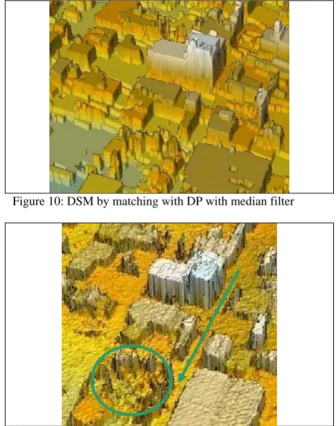
algorithms for the same area (see Figure 13) demonstrates this effect. Figure 9 demonstrates the streaking problems of DP based on IKONOS images with epipolar lines in direction of the red arrow. In the encircled location, the correct end of building could not be determined, causing a wall, closing the street. By median filtering with 1 x 5 pixels across the epipolar lines, the result of DP clearly improved (figure 10). Nevertheless some remaining streaking effects cause that the street shown in the DSM generated by SGM (figure 11) by the green arrow is disturbed and does not look like a street in figure 10. Compared to these results the DSM based on LSM is rather noisy (Figure 12).
Figure 9: DSM by matching with DP without filtering, arrow = epipolar line direction
Figure 10: DSM by matching with DP with median filter
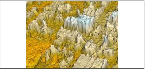
Figure 11: DSM by matching with SGM, green arrow = street International Archives of the Photogrammetry, Remote Sensing and Spatial Information Sciences, Volume XXXVIII-4/W19, 2011
Figure 12: DSM by least squares matching
Figure 13: IKONOS image of test area used for figures 9 – 12
Semi global matching is more time consuming as DP, but as demonstrated in the previous example, the DSM from SGM is clearly better as the one from DP, hence only basic tests were made with DP and it has not been used for the comparison of DSMs presented in next chapter.
On the other hand, even if the results based on least squares matching are not as good as from SGM, also tests with the LSM are included because of faster processing.
Also SGM has some limitations. In the encircled area in figure 11 low buildings are surrounded by trees (see also figure 13). In this case SGM could not detect the correct building shape, but such a situation is rare in the project area.
6. COMPARISON OF HEIGHT MODELS
6.1 Individual DSMs
As mentioned, aerial images with 7cm and with 63cm GSD from May 2007, IKONOS images with 1m GSD from May 2008 and GeoEye-1 images with 50cm GSD from September 2009 are available. The 7cm GSD aerial images also have been down sampled to 28cm GSD.
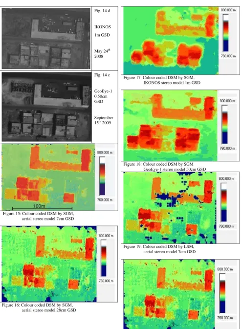
Figure 14 first gives an impression about the image quality of the different data sets. Only black-white images are shown because they have been used for image matching. The aerial images with 7cm GSD and of course also the down sampled images with 28cm GSD have a very good image quality. This is not really the case for the aerial images with 63cm GSD; they do not give a sharp impression.
The IKONOS image with 1m GSD looks better as the aerial image with 63cm GSD which is disturbed by film grain. Of
course the GeoEye-1 image with 0.50m GSD includes more details as the IKONOS image.
In the following figures 15 – 24 results from the various tests are depicted. In theses figures matching gaps are shown in dark blue. In the corresponding figure 25, the changes which have occurred during the years 2007 to 2009 are indicated.
As demonstrated with figures 23 and 24, the matching results based on aerial images with 63cm GSD are not as good as the others. Especially the DSM from LSM does not allow a determination of satisfying building shape. Only the DSM from SGM may be acceptable. The aerial images with 7cm GSD are too detailed for building monitoring – as shown in figure 14, upper image, with 7cm GSD any detail can be seen, but this is not required if only building changes shall be monitored. With 7cm GSD topographic maps larger as 1:1000 can be generated.
Figure 14: Sub-scenes of used images
Fig. 14 a
Aerial image 7cm GSD
May 25th 2007 Fig. 14 b
Aerial image down sampled to 28cm GSD
May 25th 2007
Fig. 14 c
Aerial image 63cm GSD
May 24th 2007 International Archives of the Photogrammetry, Remote Sensing and Spatial Information Sciences, Volume XXXVIII-4/W19, 2011
Fig. 14 d
IKONOS 1m GSD
May 24th 2008
Fig. 14 e
GeoEye-1 0.50cm GSD
September 15th 2009
Figure 15: Colour coded DSM by SGM, aerial stereo model 7cm GSD
Figure 16: Colour coded DSM by SGM, aerial stereo model 28cm GSD
Figure 17: Colour coded DSM by SGM, IKONOS stereo model 1m GSD
Figure 18: Colour coded DSM by SGM GeoEye-1 stereo model 50cm GSD
Figure 19: Colour coded DSM by LSM, aerial stereo model 7cm GSD
Figure 20: Colour coded DSM by LSM, aerial 28cm GSD International Archives of the Photogrammetry, Remote Sensing and Spatial Information Sciences, Volume XXXVIII-4/W19, 2011
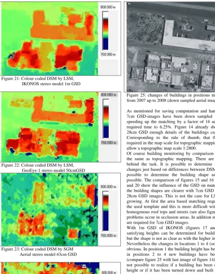
Figure 21: Colour coded DSM by LSM, IKONOS stereo model 1m GSD
Figure 22: Colour coded DSM by LSM, GeoEye-1 stereo model 50cmGSD
Figure 23: Colour coded DSM by SGM Aerial stereo model 63cm GSD
Figure 24: Colour coded DSM by LSM Aerial stereo model 63cm GSD
Figure 25: changes of buildings in positions marked by 1 – 4 from 2007 up to 2008 (down sampled aerial image)
As mentioned for saving computation and handling time, the 7cm GSD-images have been down sampled to 28cm GSD, speeding up the matching by a factor of 16 and reducing the required time to 6.25%. Figure 14 already showed that with 28cm GSD enough details of the buildings can be identified. Corresponding to the rule of thumb, that 0.1mm GSD is required in the map scale for topographic mapping these images allow a topographic map scale 1:2800.
Of course building monitoring by comparison of DSM is not the same as topographic mapping. There are different ideas behind the task. It is possible to determine the location of changes just based on differences between DSMs, but it is also possible to determine the building shape as accurately as possible. The comparison of figures 15 and 16 with figures 19 and 20 show the influence of the GSD on matching. By SGM the building shapes are clearer with 7cm GSD images as with 28cm GSD images. This is not the case for LSM with region growing. At first the area based matching requires contrast in the used template and this is more difficult with 7cm GSD on homogenous roof tops and streets (see also figure 25) and more problems occur in occlusion areas. In addition more seed points are required for 7cm GSD images.
With 1m GSD of IKONOS (figures 17 and 21) building satisfying heights can be determined for building monitoring, but the shape is not as clear as with the higher image resolution. Nevertheless the changes in locations 1 to 4 (see figure 25) are obvious. In position 1 the building height has been changed and in positions 2 to 4 new buildings have been taken town (compare figure 25 with last image of figure 14). Of course it is not possible to realize if a building has been extended in the height or if it has been turned down and built up again in the same position with larger building height, but this may be also difficult in the field. With the higher resolution of GeoEye-1 of course the result is better as with IKONOS. The building shape is clearer and more accurate (see figures 19 and 22).
As expected, with the area based LSM the building shape cannot be determined as well as with the pixel based SGM. A template size of 10 x 10 pixels led to optimal results with LSM. With smaller templates the matching success was reduced drastically and with larger template size the building shape was not as good.
6.2 Building monitoring
The DSM differences of the IKONOS DSM minus the DSMs based on the aerial images with 7cm and 28cm GSD determined International Archives of the Photogrammetry, Remote Sensing and Spatial Information Sciences, Volume XXXVIII-4/W19, 2011
by SGM (figures 26 and 27) clearly show the change of the buildings (locations 1 to 4 in figure 25).
Figure 26: DSM differences – IKONOS minus aerial 7cm GSD
Figure 27: DSM differences – IKONOS DSM minus aerial photo DSM with 28cm GSD, DSM based on SGM
Figure 28: DSM differences – GeoEye-1 DSM minus IKONOS DSM based on SGM
Figure 29: DSM differences – GeoEye-1 DSM – aerial image 28cm GSD DSM based on SGM
There are some data gaps (indicated in dark blue) and also some incorrect information on top of the buildings and close to facades. Nevertheless together with the shape of the buildings, the identification of the building changes is correct.
The lower resolution of IKONOS explains why there is more or less no difference of both differential DSMs in figures 26 and 27, using the aerial images with 7cm GSD and 28cm GSD. When comparing the IKONOS and the GeoEye results, from May 2008 to September 2009 in the area used for figures 26 and 27 no building change occurred, correctly reflected in the result, see figure 28. Only on the left side of the extended area a new building has been erected. The other height differences can be explained by occlusions and viewing shadows.
Up to now only details of the height models are shown. An overview over the whole test area give figures 30 and 31. GeoEye as well as the aerial stereo model with 63cm GSD cover approximately the same area as IKONOS.
In the following the building changes in the smaller area covered by the stereo model 2005/2003 of the aerial images with 7cm are shown in detail (see also figure 32).
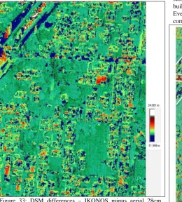
The DSM differences (figures 33-35) based on LSM show strong noise in the area of the highway and the major road marked by white lines in figure 35. Here the height models are disturbed by moving cars, low contrast and specular reflection. However, traffic areas (if known) are not important for building monitoring and the shape of groups of neighboured similar height differences is usually not confused with building changes.
The DSM based on the aerial images with 28cm GSD is not as smooth as the DSMs based on IKONOS and GeoEye-1. This can be seen at the DSM differences between GeoEye-1 and
Figure 30: Colour coded DSM by LSM of the whole area based on IKONOS stereo pair
Figure 31: Colour coded DSM by LSM of the whole area based on GeoEye-1 stereo pair
Figure 32: Area used for following building monitoring marked by red line
IKONOS in figure 34 which is not as noisy as the other one. Of course height differences at building corners caused by occlusions and viewing shadows cannot be avoided, but the colour coded height differences together with the shape indicate precisely the changes of the buildings. Even with changes of height models based on LSM, which are not as accurate in shape as the height models based on SGM, a building monitoring is possible.
Figure 33: DSM differences – IKONOS minus aerial 28cm GSD, based on LSM
Figure 34: DSM differences – GeoEye-1 minus IKONOS
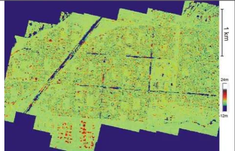
Figure 36 shows the building changes of the whole project area from May 2008 to September 2009 in red. Obvious is the new settlement in the southern part, but in the whole area new buildings have been erected or have been enlarged in height. Even the filling height of the circular tanks in the north-east corner can be seen. The scale of the DSM differences in figure
Figure 35: DSM differences – GeoEye-1 minus aerial 28cm GSD, based on LSM with marked building changes
36 is not satisfactory for determining details, it is supposed to only give an overview. More details can be seen in the enlarged figure 37. As in figure 34 the shape of unchanged buildings usually can be seen with green and orange lines caused by the different resolution of GeoEye-1 and IKONOS images and different occlusions. For the building monitoring only the solid red areas are important. The height of the new buildings or the height changes are indicated by the colour, for example the dark red colour dominating in the new southern settlement corresponds to 12m building height, while the orange colour corresponds to 5.5m.
It is difficult to specify the accuracy of the differences of the height models. Horizontal shifts have to be respected in advance if the orientation of the satellite images has not been supported by ground control points. This was done with the Hannover program DEMSHIFT, determining the shifts by iterative adjustment with satisfying accuracy quite below the GSD. In any case the relative accuracy of the DSMs against each other is important. An existing shift in height can be respected with an optimal colour table for the DSM differences. The accuracy of an individual height point is dominated by the object contrast and the 3D-shape of the surrounding area. A relative standard deviation of height differences in the range of 0.5 GSD (largest GSD used for both compared height models) multiplied with the given height to base relation is possible and realistic for areas with satisfying contrast in a planar surface. But several regions have poor contrast and as it is obvious at the shown DSM differences in the area close to building facades larger height differences cannot be avoided. SGM has a more complex situation for the accuracy of the individual height points; its standard deviation depends upon the contrast at building edges because for roofs without contrast the height is the same as for the edge in the neighbourhood. This is the same for ground areas having no contrast, but here the height situation may be more complex as for roofs, which are dominating flat in the project area.
Figure 36: DSM differences – GeoEye-1 minus IKONOS based on LSM, whole project area
For building monitoring the individual standard deviation is not important, instead it is the combination of height differences and the shape of the surrounding points with similar height differences. For the situation of the project area a height change of one floor, corresponding to approximately 2.6m, may be detectable, in any case a height change of two floors can be seen. In the open areas of the height model differences based on IKONOS and GeoEye, determined by LSM, (figure 37), the variation of the height differences is in the range of approximately +/-0.5m, indicating even a better accuracy as
mentioned before. This is the same for the top of larger buildings, but it is more complex for the areas close to the building facades as mentioned by the visible shape of unchanged buildings. In the area of streets and highways the image matching has problems with low or even non-existing contrast, specular reflection and moving cars. Such areas have to be excluded.
For SGM the variation of differences of height models are also in the range of +/-0.5m for flat ground and flat building tops. The SGM has the advantage against LSM that the building shape is more accurate; reducing also the problems close to the location of the facades.
7. CONCLUSIONS
A building monitoring by comparing digital surface models from different time periods allowed a reliable detection of all height changes of one floor or more based on aerial photos with 0.28m GSD, an IKONOS stereo pair with 1m GSD and a GeoEye-1 stereo pair with 0.5m GSD. Using semiglobal matching the building shape is accurate in the range of 2 up to 4 GSD, using LSM a smoothing effect occurs.
Another essential advantage of SGM is the fact that in contrast to LSM no initial information, e. g. in the form of seed points, is required.
For more accurate requirement of building shape, the building monitoring by DSM differences should be used to identify the location of changes and extract the building shape from the images directly. This also can be done by an automatic procedure.
The photos with the scale 1:45000, scanned with 0.63cm GSD, are not as good as the other images they have led to worse results as the IKONOS images with 1m GSD. This is a problem of scanned photos, disturbed by film grain and low contrast. With original digital aerial images such problems should not occur.
8. REFERENCES
Alobeid, A., Jacobsen, K., Heipke, C., 2010: Comparison of
Matching Algorithms for DSM Generation in Urban Areas from IKONOS Imagery, PERS 76(9). pp. 1041 – 1050.
Birchfield, S., Tomasi, C., 1998: A pixel dissimilarity measure that is insensitive to image sampling. IEEE Transactions on Pattern Analysis and Machine Intelligence, 20(4):401-406. Hirschmüller, H., 2008: Stereo Processing by Semiglobal Matching and Mutual Information, IEEE Transactions on Pattern Analysis and Machine Intelligence, 30(2):328-34. Jacobsen, K., 2008: Tells the number of pixels the truth? – Effective Resolution of Large Size Digital Frame Cameras, ASPRS 2008 Annual Convention, Portland