DEFINING SIMPLE nD OPERATIONS BASED ON PRISMATIC nD OBJECTS
K. Arroyo Ohori*, H. Ledoux, J. Stoter
3D Geoinformation, Delft University of Technology, Delft, the Netherlands — (g.a.k.arroyoohori, h.ledoux, j.e.stoter)@tudelft.nl
KEY WORDS: nD GIS, prismatic polytopes, extrusion
ABSTRACT:
An alternative to the traditional approaches to model separately 2D/3D space, time, scale and other parametrisable characteristics in GIS lies in the higher-dimensional modelling of geographic information, in which a chosen set of non-spatial characteristics, e.g. time and scale, are modelled as extra geometric dimensions perpendicular to the spatial ones, thus creating a higher-dimensional model. While higher-dimensional models are undoubtedly powerful, they are also hard to create and manipulate due to our lack of an intuitive understanding in dimensions higher than three. As a solution to this problem, this paper proposes a methodology that makes nD object generation easier by splitting the creation and manipulation process into three steps: (i) constructing simple nD objects based on nD prismatic polytopes—analogous to prisms in 3D—, (ii) defining simple modification operations at the vertex level, and (iii) simple postprocessing to fix errors introduced in the model. As a use case, we show how two sets of operations can be defined and implemented in a dimension-independent manner using this methodology: the most common transformations (i.e. translation, scaling and rotation) and the collapse of objects. The nD objects generated in this manner can then be used as a basis for an nD GIS.
1. INTRODUCTION
The traditional approaches to model 2D/3D space, time and scale in GIS are mostly based on adaptations to well-known 2D data structures, such as the DCEL (Muller and Preparata, 1978) and the quad-edge (Guibas and Stolfi, 1985). Many ‘3D’ GIS inter- nally represent objects using a 2.5D structure, essentially treating the third dimension as an attribute, or represent individual 3D ob- jects only implicitly through the 2D surface that separates their interior from their exterior. Spatiotemporal GIS keep multiple representations of 2D structures (Armstrong, 1988), each at a dif- ferent point in time, or a list of changes per object (Worboys, 1992; Peuquet, 1994), while multi-scale datasets generally con- sist of independent datasets at each scale with some identifiers that link equivalent objects between datasets (Friis-Christensen and Jensen, 2003; Stoter et al., 2014).
An alternative to this approach lies in the higher-dimensional modelling of geographic information (Arroyo Ohori, 2016), where a chosen set of non-spatial characteristics, e.g. time and scale (van Oosterom and Stoter, 2010), are modelled as true ge- ometric dimensions in addition to the spatial ones. For instance, the complete history of a set of 3D objects in time and all of their possible representations at various scales can be modelled as a single 5D model. Mathematically, a higher-dimensional model corresponds to the definition of an n-dimensional cell complex (Section 2.1), which can be directly implemented in a computer using a variety of data structures.
Higher-dimensional models are undoubtedly space-intensive, but they are also very powerful: they provide a simple and consistent way to store the geometry, attributes and topological relationships between any objects of any dimension. However, one of the main problems of higher-dimensional models is that they are not intu- itive. While we are used to solving problems in 2D and 3D, and we thus have an intuitive understanding of 2D and 3D space, and of operations on 2D and 3D objects (e.g. the Euler operators typ- ically used to create polyhedra), we do not have similar intuitive notions and experiences for nD objects.
As a partial solution to this problem, this paper proposes to use nD prismatic polytopes—analogous to prisms in 3D—as a base
* Corresponding author
for the creation and manipulation of nD models. Prismatic poly- topes essentially represent objects that are unchanged along a sin- gle dimension. By applying a modification operation to the ver- tices of the top or bottom facet of a prismatic polytope, they can be used to model many common geographic phenomena, such as objects that are moving and/or changing shape in time, or being generalised as their LOD is reduced. Moreover, unlike arbitrary nD objects, nD prismatic polytopes can be easily created based on nD extrusion, as is explained in Section 2.2.
Our methodology (Section 3) splits the creation or modification of a set of nD objects into three steps: (i) creating simple nD ob- jects based on nD prismatic polytopes, (ii) defining simple mod- ification operations at the vertex level, and (iii) simple postpro- cessing to fix the errors introduced in the model.
Within this paper, we describe in detail two concrete examples of operations defined based on our general methodology: the most common transformations applied to GIS objects (i.e. translation, scaling and rotation) in Section 4.1, and collapsing cells in Sec- tion 4.2. We finish the paper with a discussion on the possibilities of these and other nD operations based on the same methodology in Section 5.
2. RELATED WORK
2.1 nD cell complexes and their implementation
Hereafter follows a simple intuitive definition of n-dimensional cell complexes and their related terms as used in this paper. More correct (but harder) definitions are usually based on induction. See e.g. Fomenko (1990) or Hatcher (2002).
An n-dimensional cell complex is a structure made of connected cells of dimensions from zero up to n, where an i-dimensional cell (i-cell), 0 ≤ i ≤ n, is an object homeomorphic to an open i-ball (i.e. a 0D point, 1D open arc, 2D open disk, 3D open ball, etc.)1 . 0-cells are commonly known as vertices, 1-cells as edges, 2-cells as faces and 3-cells as volumes. For GIS purposes and considering only linear geometries, 0-cells are used to model points, 1-cells to model line segments, 2-cells to model polygons,
3-cells to model polyhedra, and so on. Figure 1 shows a diagram-matic description of a set of three simple polygons as a 2D cell complex.
(a) Polygons (b) Cell complex
Figure 1: (a) A set of polygons can be represented as (b) a 2D cell complex consisting of 0-cells (black disks), 1-cells (black lines), and 2-cells (coloured polygons).
Ani-cell (i > 0) is bounded by a structure ofj-cells,j < i, which are collectively known as itsboundary. Aj-dimensional face(j-face) of an i-cell is aj-cell,j ≤ i, that is part of the boundary of thei-cell. Afacetof ani-cell is an(i−1)-face of thei-cell, and aridgeof ani-cell is an(i−2)-face of thei-cell. A facet of a polyhedron is thus one of the polygons on its boundary, and a ridge of the polyhedron is one of the line segments on its boundary.
Various surveys describe the data structures that can be used to represent n-dimensional cell complexes ( ˇComi´c and de Flori-ani, 2012; Arroyo Ohori et al., 2015b). Possible data structures include incidence graphs (Rossignac and O’Connor, 1989; Ma-suda, 1993; Sohanpanah, 1989), Nef polyhedra (Bieri and Nef, 1988), and ordered topological models (Brisson, 1993; Lienhardt, 1994). nD combinatorial maps (Damiand and Lienhardt, 2014) are particularly promising (Arroyo Ohori et al., 2015b), as they are reasonably compact, can elegantly handle attributes for the cells of every dimension and have an excellent freely available implementation in CGAL2. They are thus used in order for the implementations developed in this paper.
2.2 Prismatic polytopes and their creation using extrusion
Aprismatic polytope3is the higher-dimensional analogue of a 2D
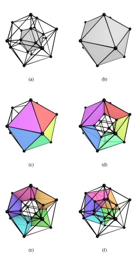
rectangle or a 3D prism. Using the terminology of a cell complex and just like in rectangles and prisms, a prismatic polytope can be defined intuitively as a cell that is bounded by a set of facets: two identical ‘top’ and ‘bottom’ facets, and a set of other facets that join corresponding ridges of the top and bottom facets. Fig-ure 2 shows an icosahedral prism, an example of a 4D prismatic polytope with icosahedron-shaped (equivalent to Figure 2b) top and bottom facets.
Extrusionis a widely used technique in GIS to construct simple 3D models from 2D+height data (Ledoux and Meijers, 2011). Starting from a set of non-overlapping polygons and a height interval associated to each of them, it generates a set of non-overlapping prisms by considering that each polygon exists all along its related interval. As shown in Figure 3, a set of building footprints and associated heights can thus be extruded into a set of simple prismatic buildings. Figure 4 shows a different 3D use case in which the third dimension represents time. The history of
2
http://www.cgal.org
3
A polytope is analogous to a polygon in 2D or polyhedron in 3D.
(a) (b)
(c) (d)
(e) (f)
a set of building footprints is thus represented by a set of extruded polyhedra.
Figure 3: A simple 3D city model created by extruding buildings.
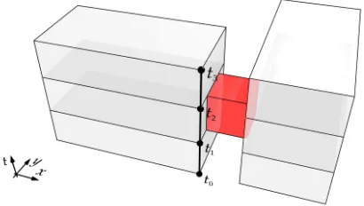
Figure 4: A 2D+time model generated using extrusion. The red volume represents the footprint of a corridor that existed between timest1andt2. The left and right building footprints were thus
extruded along[t0, t3]and the corridor footprint along[t1, t2].
While extrusion is usually used in GIS only in this 2D-to-3D form, it can be straightforwadly generalised to higher dimen-sions (Arroyo Ohori et al., 2015a): given a set of (n −1) -dimensional objects in the form of a(n−1)-dimensional cell complex, and a set of intervals per (n −1)-cell in the com-plex, it is possible to extrude the cells along then-th dimension, thus creating an-dimensional cell complex. Considering linear geometries only, this perfectly corresponds to the creation of a set ofn-dimensional prismatic polytopes from a set of(n−1) -dimensional polytopes.
When all the(n−1)-cells are extruded along a single identical interval, this operation can be computed purely combinatorially (i.e. without any geometric tests) and is equivalent to the Carte-sian product of the cells in the complex with an edge. This was described for the case of generalised maps—an ordered topolog-ical model—by Lienhardt et al. (2004). Moreover, such a pro-cedure can be repeated in order to support more than one inter-val, and given some preprocessing of the intervals by subdividing them into non-overlapping parts, it can also be used with different intervals per cell, as was suggested by Ferrucci (1993). Arroyo Ohori et al. (2015a) describes a more complex method to do so in the context of a generalised or combinatorial map, but one that minimises the total number of generated cells. For the purposes of this paper, any of these methods can be used as a base to gen-erate the required prismatic polytopes.
3. METHODOLOGY
We propose a simple methodology for the creation and manip-ulation of nD objects based on three steps: (i) an (n −1) -dimensional object or set of objects is extruded into a set ofn -dimensional prismatic polytopes, (ii) a modification operation is
applied to the vertices of the top or bottom facets of each pris-matic polytope, and (iii) simple postprocessing is used to fix the errors that were introduced in the model. The manipulation of annD object corresponds to the last two steps only. If a topo-logical data structure is used, the last step includes recomputing the topological relationships between the cells that have changed. The reasoning behind each of these steps is described in more detail below.
An-dimensional prismatic polytope, where then-th dimension represents a non-spatial characteristic such as time or scale, es-sentially representsa lack of change. It can be thus equivalent to an(n−1)-dimensional object whose geometry does not change along a period of time or whose representation is valid along an interval of levels of detail (LODs) (Arroyo Ohori et al., 2015c). While extrusion might seen unduly restrictive, it is able to pro-duce a large set of useful objects (see e.g. the complex examples in Ferrucci (1993)), and it remains simple and intuitive even in higher dimensions.
Moreover, the facets of a prismatic polytope have a few properties that make them appealing as a base for further operations:
• the top and bottom facets are parallel to the (n −1) -dimensional subspace defined by the axes of then−1 co-ordinate system of the original(n−1)-dimensional cell complex—or alternatively, the top and bottom facets are or-thogonal to the newly definedn-th axis;
• the ‘side’ facets connecting corresponding ridges of the top and bottom facets are orthogonal to the(n−1)-dimensional subspace defined by the axes of then−1coordinate system of the original(n−1)-dimensional cell complex—or alter-natively, the side facets are parallel to the newly definedn-th axis.
Together, these properties mean that it is possible to apply vari-ous modification operations by applying them directly to the ver-tices of the top or bottom facet of a prismatic polytope. Or in the case of multiple extrusions (i.e. multiple prisms stacked on top of each other), to the vertices of any facet that is orthogo-nal to then-th axis. As long as these modifications do not move the vertices of the facet out of the hyperplane4where it lies, and
the modifications do not cause the side facets to intersect (e.g. a 180◦rotation), the resulting polytope should be a reasonably
well behaved object. That is, it should contain only minor errors that are relatively easy to fix, either by minor modifications to the process or by using simple preprocessing or postprocessing steps (e.g. moving some vertices to remove self-intersections).
For instance, a smooth non-self intersecting rotation of any angle can be obtained by applying several small extrusions and rota-tions that together define the complete rotation—thus generating a screw shape rather than a twisted prism. In this manner, even rotations of more than 360◦are possible. Meanwhile, many other
types of operations causing self-intersections can be fixed by first refining the input cells into smaller cells whose neighbourhood is expected to be well-behaved. Among other examples, this pre-processing step can solve problems with flexible objects that do not morph uniformly (such as animated 3D models, which might otherwise have self-intersections), as well as non-linear transfor-mations.
4
4. TWO SETS OF OPERATIONS ON PRISMATIC POLYTOPES
In order to provide clear examples of nD operations that can be defined using the methodology described above, this sec-tion describes two such operasec-tions in detail and in a dimension-independent form: the most common transformations in Sec-tion 4.1, and collapsing cells in SecSec-tion 4.2. The former repre-sents the base of most interactive geometric modellers, while the latter together with the former provide a simple way to define a set of simple dimension-independent map generalisation opera-tors.
4.1 Simple transformations
Starting from a set ofn-dimensional prismatic polytopes, where every vertex is embedded in a location inRn, it is possible to
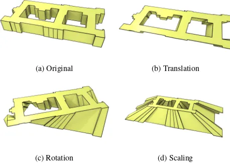
de-fine a set of basic transformations to manipulate them or parts of them (e.g. their top or bottom(n−1)-dimensional facets) simply by applying these transformations to the coordinates of their cor-responding vertices. This section thus gives a simple dimension-independent formulation of the most important transformations that are typically applied to 2D/3D objects in GIS: translation, scaling and rotation. In this way, objects that are moving or changing in shape (in certain ways) can be modelled. Figure 5 shows the result of these transformations being applied to the vertices of the top facet of a prismatic polyhedron, which was generated by extruding a building footprint with two holes. Note how the two holes in the original polygon becomegenera5of the extruded polyhedron’s surface.
(a) Original (b) Translation
(c) Rotation (d) Scaling
Figure 5: Applying transformations to the top face of (a) a prism results in: (b) a parallelepiped in the case of a translation, (c) a twisted prismin the case of a rotation, and (d) afrustumin the case of scaling.
Translatingof a set of points inRncan be easy expressed as a
sum with a vectort = [t0, . . . , tn], or alternatively as a
multi-plication with a matrix using homogeneous coordinates, which is defined as:
Plural ofgenus. Intuitively, the genus of a surface indicated how many holes or handles it has. For instance, a donut has genus 1.
For instance, it is often useful to apply a multiplication with a centering matrix(Marden, 1996,§3.2), which moves a dataset to a position around the origin. Such a matrix would be defined as
In−
1
nM1, whereInis ann×nidentity matrix andM1is an
n×nmatrix where all entries are set to 1.
Scalingis similarly simple. Given a vectors= [s0, s1, . . . , sn]
that defines a scale factor per axis (which in the simplest case can be the same for all axes), it is possible to define a matrix to scale an object as:
Rotationis somewhat more complex. Rotations in 3D are of-ten conceptualised intuitively as rotationsaround an axis. As there are three degrees of rotational freedom in 3D, combining three such elemental rotations can be used to describe any rota-tion in 3D space. Most conveniently, these three rotarota-tions can be performed respectively around thex,yandz axes, such that a point’s coordinate on the axis being rotated remains unchanged. This is a very elegant formulation, but this view of the matter is only valid in 3D.
A more correct way to conceptualise rotations is to consider them as rotationsparallel to a given plane(Hollasch, 1991), such that a point that is continuously rotated (without changing rotation direction) will form a circle that is parallel to that plane. This view is valid in 2D (where there is only one such plane), in 3D (where a plane is orthogonal to the usually defined axis of rota-tion) and in any higher dimension. Incidentally, this shows that the degree of rotational freedom innD is given by the number of possible combinations of two axes (which define a plane) on that dimension (Hanson, 1994), i.e.'n
2
(
. A general rotation in any dimension can also be seen as a sequence of elementary ro-tations, although the total number of these rotations that need to be performed increases significantly.
Consider the 2D rotation matrixRxy that rotates points inR 2
parallel to thexyplane:
Rxy=
cosθ −sinθ sinθ cosθ
*
Based on it, it is possible to obtain the three 3D rotation matrices to rotate points inR3 around the x, y and z axes, which cor-respond to the rotations parallel to the yz, zxand xyplanes6.
These would consist of an identity row and column that preserves the coordinate of a particular axis and rotates the coordinates of the other two, resulting in the following three 3D rotation matri-ces:
6
Ryz =
Similarly, in a 4D coordinate system defined by the axesx,y,z andw, it is possible to define six 4D rotation matrices, which cor-respond to the six rotational degrees of freedom in 4D (Hanson, 1994). These respectively rotate points inR4
parallel to thexy, xz,xw,yz,ywandzwplanes:
This scheme of a set of elementary rotations can be easily ex-tended to any dimension, always considering a rotation matrix as a transformation that rotates two coordinates of every point and maintains all other coordinates. An alternative to this could be to apply more than one rotation at a time (van Elfrinkhof, 1897). However, for an application expecting user interaction, it might be more intuitive to rely on an arbitrarily defined rotation plane that does not correspond to specific axes, e.g. by defining such a plane through a triplet of linearly independent points (Hanson, 1994).
Unlike the cases of translation and scaling presented above, a ro-tation applied to the vertices of the top or bottom facet of a pris-matic polytope causes its side facets to deform. The vertices of such side facets thus do not lie on a hyperplane (i.e. its vertices become non-collinear, non-coplanar, etc.). If this is a problem, it is then necessary to apply a simple postprocessing step that subdi-vides the side facets into simplices (i.e. triangles in a 3D model, tetrahedra in a 4D model). Since the side facets of model are combinatorially equivalent to(n−1)-cubes, they can be decom-posed into simplices with ease. For instance, a square is split into two triangles by an edge that joins two of its opposite vertices, and a cube can be split into 5 tetrahedra. Similar optimal simpli-cial decompositions are known up to 7D (Hughes and Anderson, 1996), while non-optimal solutions are known for any dimension (Orden and Santos, 2003; Haiman, 1991).
4.2 Collapsing cells
Collapsing cells is perhaps the most common simplification oper-ation used in both geometric processing and in cartographic gen-eralisation (Weibel, 1997). For instance, collapsing edges and
faces in a triangulation are the two most important fundamen-tal operations used in the simplification of a GIS TIN, or more generally any triangular or polygonal mesh (Hoppe, 1996). Simi-larly, roads are collapsed from areas to lines and cities are col-lapsed from areas to points at appropriate scales according to various cartographic rules (SGK, 1975). For instance, Good-child (2001) suggests a minimal feature size in paper maps of 0.5 mm—arguably, objects smaller than this value should be either increased in size or collapsed to points and represented instead using appropriate symbols.
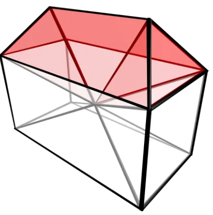
Within the methodology described in this paper, implementing the collapse of a cell of any dimension is quite simple and can be performed in three steps: (i) all the vertices of the cell are moved to a single location (e.g. the centroid of the cell or a point known to lie in its interior), (ii) the degenerate cells produced by this process are removed, and (iii) any non linear geometries that were generated are subdivided. Figure 6 shows an example with the collapse operation applied to the top face and an edge of the top face of a polyhedron. Figure 7 shows a 4D example where the collapse operation is applied to a volume.
(a) Face collapse
(b) Edge collapse
Figure 6: Cells can be collapsed by moving all of their vertices to the same location. Shown here are the collapse of (a) a face and (b) an edge on the top facet of the prism. The modified edges in (b) are highlighted in red. Note how among the modified edges, one edge that is not incident to the collapse vertex (plus another one hidden from this view) is added in order to triangulate a non-planar facet.
Figure 7: Collapsing a facet consisting of the volume of a simple 3D model of a house in 4D. As in Figure 2, the fourth dimension corresponds to an inwards-outwards axis due to the stereographic projection that is used.
Collapse operations can be used in other ways as well. As shown in the edge collapse example in Figure 6b, it is possible to de-fine operations that are applied only to certain vertices of a facet. However, these vertices do not have to correspond to the vertices of any given cell. For instance, they can be applied to the vertices surrounding a hole in the top or bottom facet. This makes it pos-sible to define operations that correspond to the removal of a hole of any dimension, such as in the example in Figure 8.
Once a collapse operation has been performed, it is then often de-sirable to remove the degenerate cells from the model, i.e. those that are infinitesimally small but still exist in the model. Such cells are those that have been explicitly collapsed, as well as the lower-dimensional ones that lie on their boundaries. However, even if this information is lost in the process, detecting the de-generating cells created by this method is straightforward: such cells are those that have all their vertices at the same location in
Rn
. An algorithm can thus iterate over all the vertices of all the cells of the model and easily find those that are degenerate.
When a topological data structure is not used, the degenerate cells can be deleted directly. However, when a topological data struc-ture is used, it is better to remove these cells using algorithms that operate on a combinatorial level and recomputes only the topological relationships that have changed. The exact form of such operations depends on the specific data structure that is used. For instance,n-dimensional combinatorial and generalised maps already have a defined dimension-independentremovaloperator (Damiand and Lienhardt, 2003, 2014) that corresponds exactly to this requirement.
If such an operation has not been defined, an alternative approach would be to remove all the combinatorial primitives belonging to the deleted cells (and are not used elsewhere), and then proceed to recompute reconstruct an object from its boundary, e.g. using the incremental construction method presented in Arroyo Ohori et al. (2014).
(a) Viewed from the top
(b) Viewed from the bottom
Figure 8: Collapsing the vertices surrounding both of the holes on the bottom facet of a prism. Note how in (b) the view from the bottom, the holes are collapsed into single vertices. If a sub-sequent extrusion was applied to this face, they could then be ignored and reflect a smoothly changing geometry.
5. CONCLUSIONS
Defining operations that are both dimension-independent and in-tuitive to use can be difficult, as we do not have the same inin-tuitive understanding of the manipulation of higher-dimensional objects that we have in 2D and 3D. Our proposed solution to this prob-lem is to define some of such operations on the basis ofprismatic polytopes, as thesenD objects are general enough to represent many phenomena commonly modelled in GIS but still have a simple geometry that is analogous to familiar shapes—2D rect-angles and 3D prisms.
Prismatic polytopes can be easily generated using dimension-independent extrusion (Arroyo Ohori et al., 2015a), and much as in 2D, extrusion is particularly appealing because it has a sim-ple definition and a relatively easy imsim-plementation in arbitrary dimensions. Starting from a set of non-overlapping (n−1) -dimensional objects, extrusion guarantees that its output consists of a set of valid non-intersectingn-dimensional objects.
shape, while the latter can be used as a basis fornD generalisa-tion, or when used together with time to model smooth anima-tions between various timestamps.
While we have only shown in this paper three concrete examples ofnD transformations (translation, rotation and scale), it is good to point out that the same scheme readily extends to other affine transformations, such as shears, reflections and homothetic trans-formations.
Within this paper, we limit the description of the operations to the top and bottom facets of a prismatic polytope, as this type of operations has a clear and intuitive meaning. However, the gen-eral methodology can be applied to any given facet of a prismatic polytope, as well as to any bounding cell of a general polytope as long as more strict constraints are kept, e.g. preserving certain relationships to the higher-dimensional cells bounded by it and avoiding intersections caused by misplacing a collapsed point.
An interesting future possibility is to consider how to intuitively define various operations as types ofreverse collapses. In ad-dition to collapsing a set of vertices to a single point, it is also possible toexpanda single vertex into an arbitrary cell of any di-mension higher than zero. In many instances, an expansion of a vertex into ani-cell is trivial to build, as it geometrically results in an(i+ 1)-dimensional pyramid with thei-cell as its base and the vertex as its apex, as can be seen by considering an operation that undoes the collapses in Figures 6a, 7 and 8. This is always true when the resulting pyramid lies completely inside or completely outside the model (i.e. the cell complex).
However, if the vertex and the expansioni-cell lie on the bound-ary of the model7, the operation is much more complex to imple-ment and in some cases can be ambiguous—thus requiring more information from the user is needed in order to form the desired combinatorial structure. This can be seen by trying to define an operation that reverses the collapse in Figure 6b. Such an opera-tion would expand the collapse vertex into an edge, but in order to do so, it would need to know which of the three triangles should be transformed into a quadrangle.
In the future, we plan to devise a more complete set of opera-tions that provide all basic funcopera-tions required in 3D+time and 3D+scale modelling while remaining intuitive, as well as to im-plement proofs of concept based on CGAL combinatorial maps.
ACKNOWLEDGEMENTS
This research is supported by the Dutch Technology Foundation STW, which is part of the Netherlands Organisation for Scientific Research (NWO), and which is partly funded by the Ministry of Economic Affairs (Project code: 11300).
References
Armstrong, M. P., 1988. Temporality in spatial databases. In: GIS/LIS ’88 : proceedings : accessing the world : third annual International Conference, Exhibits, and Workshops, American Society for Photogrammetry and Remote Sensing, pp. 880– 889.
Arroyo Ohori, K., 2016. Higher-dimensional modelling of geo-graphic information. PhD thesis, Delft University of Technol-ogy.
7
This happens when the vertex andi-cell are collinear fori = 1, coplanar fori= 2and more generally when the vertices of thei-cell and the other vertex are not linearly independent.
Arroyo Ohori, K., Damiand, G. and Ledoux, H., 2014. Con-structing an n-dimensional cell complex from a soup of (n-1)-dimensional faces. In: P. Gupta and C. Zaroliagis (eds), Ap-plied Algorithms. First International Conference, ICAA 2014, Kolkata, India, January 13-15, 2014. Proceedings, Lecture Notes in Computer Science, Vol. 8321, Springer International Publishing Switzerland, Kolkata, India, pp. 37–48.
Arroyo Ohori, K., Ledoux, H. and Stoter, J., 2015a. A dimension-independent extrusion algorithm using generalised maps. In-ternational Journal of Geographical Information Science 29(7), pp. 1166–1186.
Arroyo Ohori, K., Ledoux, H. and Stoter, J., 2015b. An evalua-tion and classificaevalua-tion of nD topological data structures for the representation of objects in a higher-dimensional GIS. Inter-national Journal of Geographical Information Science 29(5), pp. 825–849.
Arroyo Ohori, K., Ledoux, H., Biljecki, F. and Stoter, J., 2015c. Modelling a 3D city model and its levels of detail as a true 4D model. ISPRS International Journal of Geo-Information 4(3), pp. 1055–1075.
Bieri, H. and Nef, W., 1988. Elementary set operations withd -dimensional polyhedra. In: H. Noltemeier (ed.), Computa-tional Geometry and its Applications, Lecture Notes in Com-puter Science, Vol. 333, Springer Berlin Heidelberg, pp. 97– 112.
Brisson, E., 1993. Representing geometric structures in d dimen-sions: topology and order. Discrete & Computational Geome-try 9, pp. 387–426.
ˇ
Comi´c, L. and de Floriani, L., 2012. Modeling and Manipulat-ing Cell Complexes in Two, Three and Higher Dimensions. Lecture Notes in Computational Vision and Biomechanics, Vol. 2Number 2, Springer, chapter 4, pp. 109–144.
Damiand, G. and Lienhardt, P., 2003. Removal and contrac-tion forn-dimensional generalized maps. In: Proceedings of the 11th Discrete Geometry for Computer Imagery, Vol. 2886, pp. 408–419.
Damiand, G. and Lienhardt, P., 2014. Combinatorial Maps: Ef-ficient Data Structures for Computer Graphics and Image Pro-cessing. CRC Press.
Ferrucci, V., 1993. Generalised extrusion of polyhedra. In: 2nd ACM Solid Modelling ’93, ACM, pp. 35–42.
Fomenko, A., 1990. Variational Problems in Topology: The Ge-ometry of Length, Area and Volume. CRC Press.
Friis-Christensen, A. and Jensen, C. S., 2003. Object-relational management of multiply represented geographic entities. In: Proceedings of the 15th International Conference on Scientific and Statistical Database Management, IEEE Computer Soci-ety, pp. 150–159.
Goodchild, M. F., 2001. Metrics of scale in remote sensing and GIS. International Journal of Applied Earth Observation and Geoinformation 3(2), pp. 114–120.
Guibas, L. J. and Stolfi, J., 1985. Primitives for the manipula-tion of general subdivisions and the computamanipula-tion of Voronoi diagrams. ACM Transactions on Graphics 4(2), pp. 74–123.
Haiman, M., 1991. A simple and relatively efficient triangulation of the n-cube. Discrete & Computational Geometry 6, pp. 287– 289.
Hatcher, A., 2002. Algebraic Topology. Cambridge University Press.
Hollasch, S. R., 1991. Four-space visualization of 4D objects. Master’s thesis, Arizona State University.
Hoppe, H., 1996. Progressive meshes. In: Proceedings of SIG-GRAPH 1996, pp. 99–108.
Hughes, R. B. and Anderson, M. R., 1996. Simplexity of the cube. Discrete Mathematics 158, pp. 99–150.
Ledoux, H. and Meijers, M., 2011. Topologically consistent 3D city models obtained by extrusion. International Journal of Geographical Information Science 25(4), pp. 557–574.
Lienhardt, P., 1994. n-dimensional generalized combinatorial maps and cellular quasi-manifolds. International Journal of Computational Geometry and Applications 4(3), pp. 275–324.
Lienhardt, P., Skapin, X. and Bergey, A., 2004. Cartesian prod-uct of simplicial and cellular strprod-uctures. International Journal of Computational Geometry and Applications 14(3), pp. 115– 159.
Marden, J. I., 1996. Analyzing and Modeling Rank Data. CRC Monographs on Statistics & Applied Probability, Vol. 64, Chapman & Hall.
Masuda, H., 1993. Topological operators and Boolean op-erations for complex-based non-manifold geometric models. Computer-Aided Design.
Muller, D. E. and Preparata, F. P., 1978. Finding the intersection of two convex polyhedra. Theoretical Computer Science 7(2), pp. 217–236.
Orden, D. and Santos, F., 2003. Asymptotically efficient triangu-lations of the d-cube. Discrete & Computational Geometry 30, pp. 509–528.
Peuquet, D. J., 1994. It’s about time: A conceptual framework for the representation of temporal dynamics in geographic in-formation systems. Annals of the Association of American Geographers 84(3), pp. 441–461.
Rossignac, J. and O’Connor, M., 1989. SGC: A dimension-independent model for pointsets with internal structures and incomplete boundaries. In: M. Wosny, J. Turner and K. Preiss (eds), Proceedings of the IFIP Workshop on CAD/CAM, pp. 145–180.
SGK, 1975. Kartographische Generalisierung. Der Schweiz-erischen Gesellschaft f¨ur Kartographie.
Sohanpanah, C., 1989. Extension of a boundary representa-tion technique for the descriprepresenta-tion ofndimensional polytopes. Computers & Graphics 13(1), pp. 17–23.
Stoter, J., Post, M., van Altena, V., Nijhuis, R. and Bruns, B., 2014. Fully automated generalisation of a 1:50k map from 1:10k data. Cartography and Geographic Information Science 41(1), pp. 1–13.
van Elfrinkhof, L., 1897. Eene eigenschap van de orthogonale substitutie van de vierde orde. In: Handelingen van het 6e Nederlandsch Natuurkundig en Geneeskundig Congres, Delft, pp. 237–240.
van Oosterom, P. and Stoter, J., 2010. 5D data modelling: Full in-tegration of 2D/3D space, time and scale dimensions. In: S. I. Fabrikant, T. Reichenbacher, M. van Kreveld and C. Schlieder (eds), Geographic Information Science: 6th International Con-ference, GIScience 2010, Zurich, Switzerland, September 14-17, 2010. Proceedings, Springer Berlin Heidelberg, pp. 311– 324.
Weibel, R., 1997. Generalization of spatial data: Principles and selected algorithms. In: M. van Kreveld, J. Nievergelt, T. Roos and P. Widmayer (eds), Algorithmic Foundations of Geographic Information Systems, Lecture Notes in Computer Science, Vol. 1340, Springer Berlin Heidelberg, pp. 99–152.