Full Terms & Conditions of access and use can be found at
http://www.tandfonline.com/action/journalInformation?journalCode=ubes20
Download by: [Universitas Maritim Raja Ali Haji], [UNIVERSITAS MARITIM RAJA ALI HAJI
TANJUNGPINANG, KEPULAUAN RIAU] Date: 11 January 2016, At: 21:00
Journal of Business & Economic Statistics
ISSN: 0735-0015 (Print) 1537-2707 (Online) Journal homepage: http://www.tandfonline.com/loi/ubes20
Market-Based Credit Ratings
Drew D. Creal, Robert B. Gramacy & Ruey S. Tsay
To cite this article: Drew D. Creal, Robert B. Gramacy & Ruey S. Tsay (2014) Market-Based Credit Ratings, Journal of Business & Economic Statistics, 32:3, 430-444, DOI: 10.1080/07350015.2014.902763
To link to this article: http://dx.doi.org/10.1080/07350015.2014.902763
Accepted author version posted online: 18 Mar 2014.
Submit your article to this journal
Article views: 341
View related articles
View Crossmark data
Market-Based Credit Ratings
Drew D. C
REAL, Robert B. G
RAMACY, and Ruey S. T
SAYUniversity of Chicago Booth School of Business, Chicago, IL 60637 ([email protected])
We present a methodology for rating in real-time the creditworthiness of public companies in the U.S. from the prices of traded assets. Our approach uses asset pricing data to impute a term structure of risk neutral survival functions or default probabilities. Firms are then clustered into ratings categories based on their survival functions using a functional clustering algorithm. This allows all public firms whose assets are traded to be directly rated by market participants. For firms whose assets are not traded, we show how they can be indirectly rated by matching them to firms that are traded based on observable characteristics. We also show how the resulting ratings can be used to construct loss distributions for portfolios of bonds. Finally, we compare our ratings to Standard & Poors and find that, over the period 2005 to 2011, our ratings lead theirs for firms that ultimately default.
KEY WORDS: Clustering; Credit default swaps; Default risk; Survival functions.
1. INTRODUCTION
Credit ratings are a summary of a firm’s expected future cred-itworthiness. They are commonly used to quantify the credit risk for large institutions and they play an integral role in the operations of the global financial system. For example, the Basel Accord uses credit ratings as a measure of potential losses and makes credit ratings a determinant of capital requirements for financial institutions. Credit ratings also help determine what positions financial institutions such as hedge funds and mutual funds are legally allowed to hold through contractual obliga-tions. Financial institutions may build their own ratings system or they can use the ratings systems of independent agencies (e.g., Moody’s, Standard & Poors, and Fitch).
We propose a methodology that allows the prices of traded assets to directly determine the credit ratings for publicly traded firms with a minimal amount of subjective input on a firm-by-firm basis. We call these market-based credit ratings. Our methodology uses the information available in financial markets to construct credit ratings in a transparent manner. Our credit ratings are in real-time as they only use information up to the date the rating is given. The essential element is to specify a function that maps the observed value of firms’ credit risky assets into a rating category. This function enables any public firm that is currently traded to be rated.
We begin by converting the observed prices of corporate bonds and credit derivatives into survival functions, which equal one minus the cumulative probability of default on or before a given future date. To construct market-based credit ratings, we focus directly on the survival function because it is the object that is common for traded, credit risky assets. A credit default swap (CDS) is a financial agreement between a buyer and seller that is similar to insurance and is intended to protect the buyer of the contract in case a bond or loan defaults. The buyer of the CDS contract makes periodic payments known as premiums to the seller and, in exchange, receives a payoff from the seller if the reference entity defaults on a loan or bond before the CDS contract matures. The reference entity is the organization on which the CDS contract is written and may be a municipal, state, or sovereign government or a public or private corpora-tion. The periodic payment that the buyer makes to the seller
is quoted in terms of a spread. Spreads are higher for entities who the market perceives to have either higher probabilities of default or whose default has worse consequences, leading to a correspondingly greater insurance cost.
In recent years, independent ratings agencies Moody’s and Standard & Poors also allow financial institutions to purchase either ratings implied by market prices (S&P) or CDS-implied default probabilities (Moody’s). The ratings agencies, therefore, do provide a form of “market-based” rating. But the methods used in those market-based ratings are not openly available. In contrast, the emphasis in this article is developing a method that is transparent and whose function mapping observed asset prices into ratings is publicly known. Furthermore, our methodology will provide a market-based rating for those firms that do not have bonds/CDS traded on the market.
We take market prices and transform them into market implied survival probabilities using standard asset pricing formulas. The survival functions are then clustered into ratings categories using a “model-based” functional clustering algorithm. Importantly, the model behind the clustering algorithm is intended as a clas-sification device. It is not intended to describe the mechanism that generated the data. The output of the clustering algorithm allows us to build two types of ratings:absoluteandrelative ratings.
We define “absolute ratings” to be a classification system where each rating category has a time-invariant, precise eco-nomic definition. Absolute ratings, therefore, provide a publicly known point of reference that does not change through the credit or business cycle. During a credit crisis when short-term lending to businesses by banks dries up, it may be that few, if any, firms are able to attain the highest absolute rating. In contrast, many agency-issued credit ratings are letter grades, which do not have a precise definition.
© 2014American Statistical Association Journal of Business & Economic Statistics
July 2014, Vol. 32, No. 3
DOI:10.1080/07350015.2014.902763
Color versions of one or more of the figures in the article can be found online atwww.tandfonline.com/r/jbes.
430
We define “relative ratings” to be a classification system where the creditworthiness of an individual firm is compared to other firms at that point in time. In practice, a firm’s credit-worthiness may decline considerably during a recession but it may not decline as much as other firms meaning that the firm is relatively better off. In such a case, a firm’s relative rating may increase while its absolute rating declines. Cash-rich compa-nies such as Apple and Microsoft were good examples of firms whose relative rating increased during the recent financial crisis. Another contribution of this article is to develop a method to rate public firms whose assets are not actively traded using firms whose assets are. This amounts to solving a counterfac-tual. How would the market rate a firm if its assets were traded? Intuitively, two firms that are identical in terms of observable characteristics but only one of which is traded should receive the same or comparable credit ratings. We solve the counter-factual problem using matching estimators. Specifically, we use observable characteristics to match firms for which we do not observe debt or credit derivatives data with other firms for which we do have such data.1
We implement our methodology using a large database of daily CDS spreads from 2005 through 2011 along with the Lon-don Interbank Offered Rate (LIBOR) deposits and interest rate swaps, which we convert to survival functions. There are many arguments in the literature as to why these securities are informa-tive about default probabilities. Several papers have documented that CDS spreads lead changes in bond yields and credit ratings, for example, Hull, Predescu, and White (2004) and Blanco, Brennan, and Marsh (2005). Furthermore, CDS contracts for many reference entities are more liquid than corporate bonds as there is little initial cost to enter into a CDS contract. In fact, prior to April 2009, it was a convention in the CDS mar-ket that there was no initial cost, making it easily accessible. In addition, CDS spreads are not affected by as many detailed provisions or features associated with corporate bonds such as seniority, callability, etc. As such, CDS spreads are relatively more homogeneous than bonds across firms. As a practical mat-ter, databases on CDS spreads are more readily available and easier to manipulate than bond trades. Note, however, that be-cause our methodology works with survival functions directly, it is simple to use corporate bond data instead of, or in addition to, CDS data if it is available.
Finally, we describe how our methods can be used to con-struct loss-distributions, which are important in practice for credit risk management. Over the past decade, a large number of new models and methods have been proposed for construct-ing loss distributions, for example, Duffie and Sconstruct-ingleton (2003), Pesaran, Schuermann, and Treutler (2005), Duffie, Saita, and Wang (2007), Koopman and Lucas (2008), and Duffie et al. (2009). Our approach both complements and leverages this pre-vious research. We combine the database on CDS spreads with data from Compustat and CRSP which provides information on bankruptcies and defaults. By making default a category to which a firm can transition, we show how one can construct
1We acknowledge that firms may look identical based on observable
character-istics but differ based on firm-specific unobservable charactercharacter-istics. Assessing the credit risk of firms that have no assets traded and which differ from traded firms based on unique unobservable characteristics is a difficult task because the ratings must be determined solely by prior information.
loss distributions directly from the mixture model used to build the ratings. Alternatively, the new ratings can be used inside models for credit ratings transitions, for example, Gagliardini and Gouri´eroux (2005), Koopman, Lucas, and Monteiro (2008), Creal, Koopman, and Lucas (2013), and Creal et al. (2014).
In using our method, one should clearly ask whether, and to what extent, securities prices are informative of the underlying firm’s credit quality. The answer depends on a number of factors, most notably liquidity. Our ratings are built on a weekly basis from daily data so that day-to-day fluctuations in liquidity of the market should have a smaller impact. Using risk-neutral survival functions to construct ratings also relies on the assumption that observed spreads are not wildly distorted from fundamental values of the firms. Information does not flow through over-the-counter markets the way that it does through equity markets; see, for example, Duffie (2012). Importantly, our article does not argue that credit markets are efficient. Rather, we offer a methodology that determines ratings directly from observable data and argue that this offers a useful source of information to complement other sources, for example, ratings agencies. Moreover, the rating method used is transparent since the CDS data are readily available and the clustering algorithm standard. The rest of this article proceeds as follows. In Section2, we discuss how ratings can be constructed from observed asset pric-ing data both for firms that are traded and for firms that are not. This section takes the risk neutral survival functions as given. In Section3, we describe the details of the data. In Section4, we compare our ratings to those of independent agencies and de-scribe how our ratings can be used to construct loss functions for portfolios of bonds. We conclude and discuss some extensions in Section5.
2. CLASSIFICATION METHODOLOGIES
2.1 Model-Based Clustering of Firms
In this section, we describe a methodology for rating firms whose credit-risky assets have been traded. Providing credit ratings is equivalent to grouping firms into a small number of categories and attaching an economic meaning to each cate-gory. From a statistical perspective, credit ratings are a form of dimension reduction; that is, a summary of a large amount of information about a firm. We take a “model-based” clustering approach. Importantly, we view the model that is used to clus-ter firms together as part of the algorithm. It is not intended to represent the mechanism believed to generate the asset pricing data we observe.
We let SitQ(τ) denote the survival function under the risk-neutral measureQfor firmiat timetwith maturityτ. Further details about the data and the procedure used to constructSitQ(τ) are discussed in Section3. At the moment, we take the vector SitQ(τ) as given fort=1, . . . , T. The number of firms for which some assets are traded in period t is Nt and for each firm a
maximum of J points on the survival function are observed, that is, some points on the survival function may be missing for some firms. Elements of the survival functions are ordered in the vector in terms of a set of increasing maturities τ =
(τ1, τ2, . . . , τJ)′. In addition to the survival functions, we also
observe a default indicator Dit which is equal to 1 if firm i
defaults in periodtand zero otherwise.
2005 2006 2007 2008 2009 2010 2011 0.02
0.04 0.06 0.08 0.1 0.12 0.14 0.16
credit default swaps
20050 2006 2007 2008 2009 2010 2011
0.1 0.2 0.3 0.4 0.5 0.6 0.7 0.8 0.9 1
Risk neutral survival functions
2005 2006 2007 2008 2009 2010 2011
0 1 2 3 4 5 6 7 8
Inverse logistic transformation
0 2 4 6 8 10
0 0.1 0.2 0.3 0.4 0.5 0.6 0.7 0.8 0.9
1 survival functions vs maturity
Figure 1. Data for the Alcoa Corporation from January 2005 through February 2011. Upper left: CDS spreads for seven different maturities
τ=(0.5,1,2,3,4,5,7,10) measured in years; Upper right: market-implied survival functionsSitQ(τ); Lower left: transformed functionsyit(τ); Lower right: survival functionsSQit(τ) as a function of maturityτfor all time periods.
We propose to construct ratings categories for traded firms by clustering a transformation of their survival functionsyit(τ)=
log(SitQ(τ)/(1−SitQ(τ))). Clustering the entire survival function instead of only a portion of it (e.g., only 5-year default proba-bilities or the level, slope, and curvature) allows the data to de-termine as to which characteristics of the survival function are important.Figure 1plots the raw and transformed CDS data for the Alcoa Corporation. The figure illustrates the rapid increase in CDS spreads during the recent financial crisis as the price for buying protection against the default of Alcoa increased. Increases in CDS spreads imply an increase in the (risk-neutral) default probability of the firm as seen by the survival probabili-ties during this period.
To cluster firms, we take a model-based clustering approach using mixtures of Gaussian processes. Consider the following
finite mixture model
yit(τ)∼ K
k=0
πit,k·p(y|μk(τ), k(τ), Dt),
πit,k= K
ℓ=0
πit,ℓk, (1)
πit,ℓk=P(Iit=k|Ii,t−1=ℓ;Yit),
∀ ℓ=1, . . . , K, ∀ k=0,· · ·, K (2)
πit,00 =P(Iit=0|Ii,t−1=0;Yit)=1, (3)
where Iit is a (latent) indicator function taking values from
k=0, . . . , K while p(y|μ, ) is a constrained multivari-ate normal distribution with mean vector μ and covariance
matrix. This distribution guarantees that the ordering con-straint (∞> y1t(τ1)> y2t(τ2)>· · ·> yJ t(τJ)>−∞) is
al-ways satisfied for any realization, which is consistent with no-arbitrage.2The probabilities π are defined below. The model in Equations (1)–(3) defines a probability distribution over the space of survival functions. We define statek=0 to be default and the largest categoryKto be the best rating category. While realizationsyit(τ) are vectors of lengthJ, the unknown
param-eters μ,, and π do not depend on J. Among other things, this allows for unbalanced panels where the vectorτ may vary acrossiandt. It also helps us to cope with missing data, which we encounter in our empirical application.
The probability of transitioning from categoryℓto category kfor firmiat timetisπit,ℓk. The transition probabilities may
depend on observable firm, industry, or macroeconomic vari-ablesYit. For stateℓ=0 whenDit=1, the normal distribution
is degenerate with all its mass at the mean (such thatSitQ=0). Equation (3) ensures that default is an absorbing state and once a firm transitions into default it cannot transition out. If in the data a firm transitions out of default, we treat it as a new firm.
In our empirical work in Section 4, the transition proba-bilities are constant across firms but vary through time as a function of observable factors. Allowing the transition ma-trices to change through time enables firms to move more rapidly between ratings categories during times of deteriorat-ing market conditions. We parameterize the transition proba-bilities as log(πt,ℓk)=αℓk+βℓk′ Yt. We ensure that each row of
the transition matrix sums to one by enforcing the constraint αℓ1< αℓ2<· · ·< αℓK. An alternative model for the
probabili-vectors of all observations, default indicators, and category in-dicators. We usey1:t =(y1′, . . . , y
′
t)
′andD
1:t =(D1, . . . , Dt)′
to denote the history of all the observable variables up to timet. We also define θk =(μk,vech(k)) and θ=(θ1′, θ
to be vectors containing the parameters of the model, where vech(k) denotes the half-stacking vector of the symmetric
matrix k. Conceptually, the number of categories could be
estimated from the data; see, Fr¨uhwirth-Schnatter (2006) for a discussion of different approaches. However, we believe it is better to consider the number of categories K to be a choice variable on the part of the practitioner.
To identify the model statistically and to give an economic interpretation to the categories, structure needs to be imposed on the mean vector and covariance matrices. For any particular rating categoryk >0, the mean vectorμkis a decreasing
func-tion of maturity, that is,μk(τ1)> μk(τ2)>· · ·> μk(τJ) with
τj−1< τj forj =2, . . . , J. This stems both from the definition
of the survival functions and the absence of arbitrage. To assign an ordering to the nondefault states fork=1, . . . , K, we im-pose that better ratings categories have higher survival functions.
2In Section3, we map the raw credit default swap data into survival functions
using an asset pricing model that imposes no-arbitrage and consequently a de-clining survival function. Therefore, the survival functions automatically satisfy this constraint.
Roughly, this means that for any maturityτj and neighboring
categoriesk−1 andk, we haveμk−1(τj)< μk(τj). We explain
how we impose these restrictions below.
There exists some freedom when determining the parameters θof the model. One can a priori fix the values of the parameters and treat them as choice variables. For example, the parameters of the mean vector could be chosen to match the values of a rep-resentative company’s survival functions at key historical times, for example, they could represent American International Group (AIG), Johnson & Johnson, or Toys ‘R’ Us in a good or bad year. Then, the ratings would be endogenously determined by com-paring other firms’ survival functions to these benchmarks. At the other extreme, the parameters of the mixture model can be freely estimated subject to the restrictions discussed above.
In practice, even for small values ofK(the rating categories) andJ(the number of maturities), the parameter set can be pro-hibitively large. We strike a middle ground between the afore-mentioned two extremes and estimate some parameters of the model while imposing further restrictions. The covariance ma-trices are restricted to be the same across ratings categories. The mean vectorsμ1, . . . , μK are also restricted such that they are
collectively only a function of a small set of parameters. Specif-ically, we allow the mean vector of the highest rated category μK to be freely estimated. Then, each additional mean
vec-tor is a deterministic decreasing function of the vecvec-tor before it,μk−1(τj)=μk(τj)−1. This ensures that the components of
the mixture are well-separated and cover the full support of the space of survival functions.
With these restrictions in place, the mixture model can be estimated by a number of methods. Techniques for estimating mixture models are well-developed in the literature; see, for example, McLachlan and Peel (2000) and Fr¨uhwirth-Schnatter (2006). We employ Bayesian methods and estimate the model by Gibbs sampling using data augmentation. As the Gibbs sampling algorithm is reasonably standard, we leave details of it to the appendix.
We estimate the parameters on only a subsample of the data (i.e., a training sample) and keep them fixed. Other than an initial training period when the parameters of the model are estimated, our ratings can be constructed in real time. Our ratings do not have an informational advantage over ratings agencies such as S&P or Moody’s. They mimic the information set of an investor who at timetdoes not observe future asset prices.
Since the mixture model is a Markov-switching model, we can use well-known algorithms for computing the prediction p(It|y1:t−1, D1:t−1;θ), filteringp(It|y1:t, D1:t;θ), and
smooth-ing distributions p(It|y1:T, D1:T;θ) which are the probability
that a firm is in rating category kconditional on different in-formation sets, for example, Hamilton (1989) and Fr¨uhwirth-Schnatter (2006). This enables one to quantify the uncertainty associated with a firm’s rating and to obtain forecasts of fu-ture ratings transitions. The model-based clustering approach advocated here is also related to discriminant analysis; see, for example, Hastie, Tibshirani, and Friedman (2009). Consider the marginal filtering distribution,
Traditional linear discriminant analysis is the special case when k= for all k and the priors over categories are
time-invariant.
In the case of a Markov-switching model, the priors over each component depend on the history of a company’s past ratings. The conditional decision boundary at timetbetween any two ratings categorieskandℓis
logp(Iit=k|y1:t, D1:t;θ)
which is a linear function of the current observationsyitand a
weighted function of past observations with declining weights. Neighboring observations play an important role in smoothing the ratings intertemporally. If in the last period there was a high probability of being in categoryk, then that probability persists into this period. A user can eliminate intertemporal smoothing of ratings by simply replacing the Markov dynamics with time-invariant probabilities for each category.
2.2 Rating Firms Whose Assets are Traded
The information from the data about a firm’s credit rating is contained in the joint posterior distributionp(I0:T|y1:T, D1:T;θ).
To turn this information into credit ratings, we need to specify a decision rule that maps probabilities into indicators that are one for only one category in a given time period. This map-ping is intricately related to a researcher’s loss function. In the following, we will propose specific methods that are computa-tionally tractable and imply a specific loss function. However, we emphasize that given the distribution p(I0:T|y1:T, D1:T;θ)
other researchers may wish to use their own loss function. We view this as an advantage of this approach.
2.2.1 Absolute Ratings. The first type of market-based rat-ings we construct areabsolute ratings. In an absolute ratings system, the definition of each category is time invariant, quan-titatively explicit, and public knowledge. The absolute ratings provide a point of reference that is interpretable and compara-ble across time periods. Specifically, we associate each mixture component,k, with its own ratings category, defined by the func-tionμkwhich determines the mean default probabilities for that
category as a function of maturityτ. In this article, we parame-terize the functionsμkto ensure that ratings categories are well
separated in terms of their average default probabilities. To construct our absolute ratings, we use the maximum a posteriori (MAP) estimator, which is the set of state indicators that maximizes the joint distributionp(I0:T|y1:T, D1:T;θ). This
is the optimal decision rule under an absolute error-loss func-tion, and can be conveniently computed by the Viterbi (1967) algorithm. The MAP estimator for the joint distribution is dif-ferent than the MAP estimator for the marginal distribution as it creates intertemporal smoothing of the ratings. We run the joint MAP estimator when each new observation becomes available taking the final period’s estimate as the rating for that period. Therefore, ratings at timetonly depend on information up to that time period.
A feature of the absolute ratings system is that a firm’s credit rating does not directly depend on the rating of other firms. The number of firms in any given rating category could be zero at some points in time. This possibility makes sense. If credit ratings are intended to signal an increase in default probabilities or poor economic outcomes, then during a credit crisis like 2008–2009 there should be very few firms with the best absolute rating. If the credit market freezes and the willingness for banks to provide short-term lending to businesses deteriorates, this would affect all firms. Conversely, a massive expansion of credit through a combination of lax regulation and perverse incentives in the credit market could lead to an increase in lending to lower quality borrowers. Both of these scenarios would be observable in the time variation of the empirical distribution of the absolute ratings system.
2.2.2 Relative Ratings. Relative ratings are another useful source of information that can be defined from the output of the clustering algorithm. In a relative ratings system, a firm’s creditworthiness is compared to other firms in that time period. Therefore, relative ratings are an ordinal ranking of firms’ credit quality.
Given the information in the posterior marginal (filtering) dis-tribution, there are many ways of sorting firms intoK∗ordered categories, whereK∗ may differ from the value ofK used to estimate the model. Each sorting scheme corresponds to a loss function. We propose to sort companies intoK∗-tiles according to their expected values from the marginal filtering distribution. Specifically, we compute the expected value for each firm
¯
nies can then be sorted intoK∗different categories by ordering their expected values from smallest to largest and splitting them intoK∗groups with an equal number of firms per group.
Relative ratings have the potential to behave differently than the absolute ratings. For example, it may be the case that during a recession or credit crunch a firm’s overall creditworthiness declines considerably but it may not decline as much or as fast as other firms causing its relative rating to increase rather than decrease. This is despite the fact that its absolute rating is declining. The relative ratings for an individual firm can be compared across time periods to see how a firm is performing relative to its peers either overall or within an industry. The empirical distribution of the relative ratings of companies in an industry or subsector of the economy also provides a simple indicator of that sector’s relative performance.
2.3 Rating Firms Whose Assets are not Traded
When a firm’s debt and credit derivatives are not actively traded, financial markets do not provide a direct signal of a firm’s credit quality. A firm’s credit rating consequently cannot be directly inferred from the transactions of market participants. Instead, one must infer the market’s rating for firms that are not traded using the market prices for firms whose assets are traded. The thought experiment is as follows. Imagine two firms that are identical to one another in every way except for the fact that one firm’s assets are traded and the other is not. These firms
should have the same or similar credit quality and share the same rating.
The idea of comparing similar economic agents (in our case firms) in two states of the world is a cornerstone of the mi-croeconometrics and statistics literature on estimation of causal effects (treatment effects); see, for example, Angrist and Pis-chke (2009) and Wooldridge (2010). Imputing either the rating category or the propensity to be in a rating category is a natural extension of the literature in credit risk management that mod-els the propensity to default. The literature on default estimation and credit risk management does not explicitly use the language of treatment effects and matching estimators. However, all the models and estimators in the literature can be interpreted as matching estimators.
Consider the simplest case where we observe for each firm a sequence of default or bankruptcy indicators and a vector of covariates. Traditional analysis of these data fit a probit or logit model to the default indicators; see, for example, Shumway (2001) and McNeil, Frey, and Embrechts (2005). Firms have either received the treatment (default) or have not received the treatment (nondefault). Firms that have not defaulted but, ac-cording to the covariates look similar to firms that have, will have a large default probability. Conditional on the ratings pro-duced in Sections 2.2.1 and 2.2.2, the ratings for nontraded firms can be imputed by matching them to traded firms based on observable characteristics.
Characteristics used for matching need to be publicly ob-servable although it is possible that regulators have access to proprietary data sources which could be used as additional in-formation. Our primary resource for characteristics will be data from accounting statements. Details of the characteristics used in this article are discussed in Section 3. We assume for the moment that we have a vector of characteristicsXj t for each
firm that is traded and a vector of characteristics ˜Xit for each
firmi that is not traded, both at timet. These vectors can be separated into subvectors of discrete and continuous variables, Xj t =(Xdj t′, X
There are many possible parametric and nonparametric meth-ods that could be employed to produce matches. We use a non-parametric matching estimator from Abadie and Imbens (2006); see also Guo and Fraser (2009). Consider constructing a match for an individual firmi at timet whose assets are not traded. First, we find the set of traded firms that share any common discrete characteristics, for example, the same industry code. This causes the firm to be matched exactly along this dimen-sion. From this set we choose the firmjthat is closest to firmi according to the distance measuredij defined by
dij =X˜itc −X
whereVis a positive definite weighting matrix. There are two common choices for the matrixV. The first is the inverse of the sample variance matrix and the second is the inverse of the sample covariance matrix in which case the distance measure (4) is the Mahalanobis distance. In our empirical work below, we use the inverse of the sample variance matrix.
This matching estimator has the advantage of being simple to implement, computationally fast, and it easily handles missing values in the characteristic space ˜Xit. With a fully nonparametric
estimator, it is also possible to identify both the sets of firms that act as a match and exactly which firm is the final match. Look-ing at which firms are matched together can provide valuable information when thinking about the plausibility of the results. Using matching estimators requires making an overlap or common support assumption. This assumption states that for each entity that did not receive the treatment, its observable characteristics ˜Xit must be similar to the observable
charac-teristics of a firm that did receive the treatment. Otherwise, a sensible match cannot be constructed and we cannot infer from market data as to what the rating should be. In the context of market-based ratings, we view this as a feature of the approach. It is practically inevitable that there will exist firms that have no common characteristics with other firms. We would like to identify these firms. Clearly, their ratings will be based entirely on prior beliefs or private information.
3. DATA
3.1 Data Sources
We use a large database of daily single entity credit default swap (CDS) spreads to construct the firm level survival func-tions. The data are from Markit Corporation and include for-eign and U.S. corporations as well as soverfor-eigns, U.S. states, and U.S. county reference entities. The data cover CDS con-tracts with yearly maturitiesτj ∈ {0.5,1,2,3,4,5,7,10}some
of which may be missing. The data are, therefore, in the form of an unbalanced panel. For simplicity, we restrict attention to CDS contracts for U.S. corporations in U.S. dollars for senior subordinated debt. And, we consider only CDS spreads under the XR clause.
After making these selections, the CDS data includes 1577 U.S. corporations over the period January 3, 2005 through February 28, 2011 making for a total of 1606 days. Of these firms, 1048 are public corporations, 310 are subsidiaries, and 219 are private firms. In some cases, firms have merged or been acquired or have gone public or private. Data on mergers/ acquisitions are available from the Center for Research in Secu-rity Prices (CRSP), which is an additional data source discussed below. When any of these actions occurs, we treat the firm as a new reference entity. Finally, we build our ratings on a weekly basis (Wednesdays) from the daily data making for a total of 321 weeks over this time period. This limits the influence of daily liquidity in the CDS market on the resulting ratings.
We combine the CDS data with data on defaults, bankrupt-cies, and credit events, which are collected from three sources. Over the period of our sample, we collect all defaults from the Standard & Poors Ratings Express database for entity ratings, all bankruptcies from the CRSP database stock event files, and all credit events that triggered payments on CDS from the Markit Corporation. The formal definitions of default, bankruptcy, and credit events are not homogenous. Therefore, it is possible for a firm to exhibit any combination of the three events. Due to the rarity of these events, we will label any one of the three events as a “default.” If more than one of these events occur for a specific firm, the events may not occur on the same date and we take the earliest of the events. The first (and most common) event is typically a default or missed interest payment in the Standard
& Poors database followed by a bankruptcy in the CRSP event files and finally a credit event that triggers the payment clause in a CDS contract. For example, a firm may miss an interest payment on a loan or bond causing Standard & Poors to label it a default. However, the firm’s stock may continue trading and the firm may never declare bankruptcy. If the firm does file for Chapter 7 or 11 bankruptcy and has publicly traded equity on an exchange, the bankruptcy will appear in the CRSP stock event files when the firm becomes delisted from the exchange. Finally, if the economic event triggered the CDS, the credit event typ-ically follows a few weeks later. The reason that credit events lag the other events is because it takes a review board several weeks to rule on whether a firm did trigger the default clause in the CDS contract; see, for example, Markit (2009).
We invert a CDS pricing formula to calculate the risk neutral survival functionsSitQ(τ) following the procedure described in O’Kane (2008). This is a procedure in the finance industry called “bootstrapping” and is part of a standard method for marking to market a CDS contract.3Importantly, the methodology we pro-pose in this article treats survival functionsSQas data and does not otherwise depend on the asset pricing model one uses to ex-tract them from observed market prices. In practice, a researcher may obtain default probabilities using whichever pricing model she prefers and still apply our methodology to obtain credit ratings. Models used for pricing CDS contracts can be found in Duffie and Singleton (2003), McNeil, Frey, and Embrechts (2005) and O’Kane (2008).
Asset pricing formulas for CDS spreads require two addi-tional sources of data. The first are the daily discount factor curveszt(τ), or zero-coupon bond rates, which describe the
mar-ket value today of a dollar delivered on dayt+τ. We follow market convention for marking assets to market and construct the discount curves from daily interest rate and credit deriva-tives data. We use overnight and two-day LIBOR rates, monthly LIBOR rates with maturities from 1 to 12 months, and interest rate swaps with maturities 1 year to 10 years. The data allow us to construct the LIBOR discount curve beginning at day zero and extending to a maturity of 10 years. Both datasets were obtained from Bloomberg.
The second input in CDS pricing formulas is an assumption about the loss-given default (LGD), which is the percentage of principal that an investor loses conditional on default by a firm. This may vary from firm to firm and over the business-cycle. Data on LGDs are relatively scarce as no financial instruments are actively traded that are functions of only the LGD. When a credit event occurs and a CDS gets triggered, an auction is made to sell the residual value of any bonds. The information on LGD from the auctions is publicly available from Markit but there have only been 52 credit events for U.S. corporations over the course of our sample. Therefore, it has been a market convention to assume a value of 60% based on historical estimates collected by Moody’s and Standard & Poors. As a standard procedure in the CDS market, the Markit corporation provides LGD estimates which are used by market participants to provide quotes. We use these values in our work and if they are not available we use 60% as a default. Whether or not these are the true LGDs, the
3This type of bootstrap should not be confused with the bootstrap used in
statistics.
resulting survival functions are consistent with how the market quotes spreads.
3.2 Data for the Matching Estimators
To determine as to which firms have the potential to be rated, we download the entire Compustat and CRSP database from 2005 through 2011. After eliminating the U.S. operations of foreign firms and nonpublic financial firms that do not disclose accounting statements, there are 6933 firms reporting earnings over the period. Of these, 1048 are public firms for which CDS trades are observed during the sample. This leaves 5885 firms whose ratings need to be imputed.
We obtain characteristics for use in the matching estimators from accounting data available from Compustat and CRSP. The variables we use are taken from Altman, Fargher, and Kalotay (2011) who find evidence that these characteristics help pre-dict the variation in risk-neutral default probabilities from the Merton (1974) model. These variables include two measures of firm specific performance: the ratio of total earnings to total assets and the ratio of retained earnings to total assets. We use two measures to quantify leverage. The first is the ratio of total assets to total liabilities and the second is accounting leverage, which is total assets divided by total assets minus total liabil-ities. The debt maturity structure of a firm is measured by the log-ratio of current liabilities to noncurrent liabilities. We mea-sure relative liquidity of assets by the ratio of working capital to total assets. We also add the four digit Standard Industrial Classification (SIC) code as our industry variable, although the Global Industrial Classification (GIC) codes would be another alternative. Further details on these variables are available in the data appendix.
In theory, characteristics used for matching may be different across industries either due to data availability or to recognize the conventional wisdom that some variables are more relevant in some sectors of the economy than others. For example, banks have different accounting standards than nonbanks and they do not report working capital or current liabilities. Credit risk for financial institutions is often associated with the composition of their balance sheets and the liquidity of their assets. Banks do not publicly release detailed information but they are required to submit “call reports” that provide some information on their holdings.
In practice, when implementing the nonparametric matching estimator, we start by using the four-digit SIC code and, if less than five matches exist at the four digit code, we work backward to the three digit SIC code. If there are less than five matches at the three digit code, we then work back to the two digit code, etc. Throughout our work, we time the arrival of the covariates to coincide with the day earnings are reported by each firm. Our goal is to mimic the information set available to the market. In between reporting dates, we take the last reported data from the earnings statement as the current value of the characteristic, which implies thatXitis a step function.
4. EMPIRICAL RESULTS
4.1 Ratings
We construct the absolute and relative ratings by running the clustering algorithms outlined in Section2.1and the matching
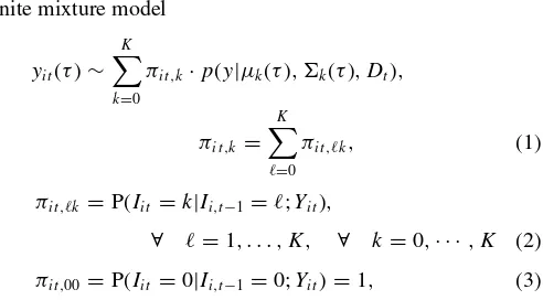
Table 1. Estimation results for the mean vectors of the survival function
μS
1 μ
S
2 μ
S
3 μ
S
4 μ
S
5 μ
S
6 μ
S
7 μ
S
8 μ
S
9
τ1
2 0.7836 0.9078 0.9640 0.9864 0.9950 0.9981 0.9993 0.9997 0.9999
(4.24e−4) (2.09e−4) (8.68e−5) (3.33e−5) (1.25e−5) (4.60e−6) (1.70e−6) (6.00e−7) (2.00e−7) τ1 0.5870 0.7944 0.9131 0.9662 0.9873 0.9953 0.9983 0.9994 0.9998
(5.55e−4) (3.74e−4) (1.82e−4) (7.48e−5) (2.88e−5) (0.12e−5) (4.00e−6) (1.50e−6) (5.00e−7) τ2 0.3230 0.5646 0.7790 0.9055 0.9630 0.9861 0.9948 0.9981 0.9993
(4.66e−4) (5.24e−4) (3.67e−4) (1.82e−4) (7.58e−5) (2.92e−5) (1.10e−5) (4.10e−6) (1.50e−6) τ3 0.1902 0.3897 0.6344 0.8251 0.9277 0.9721 0.9896 0.9961 0.9986
(3.13e−4) (4.84e−4) (4.72e−5) (2.94e−5) (1.37e−5) (5.52e−6) (2.10e−5) (0.08e−7) (2.90e−6) τ4 0.1211 0.2725 0.5046 0.7346 0.8827 0.9534 0.9823 0.9934 0.9976
(2.11e−4) (3.93e−4) (4.96e−4) (3.86e−4) (2.05e−4) (8.80e−5) (3.44e−5) (1.29e−5) (4.80e−6) τ5 0.0829 0.1972 0.4003 0.6447 0.8314 0.9306 0.9733 0.9900 0.9963
(1.49e−4) (3.10e−4) (4.71e−4) (4.49e−4) (2.75e−4) (1.27e−5) (5.10e−5) (1.94e−5) (7.20e−6)
τ7 0.0497 0.1245 0.2788 0.5124 0.7407 0.8859 0.9548 0.9829 0.9936
(9.22e−5) (2.13e−4) (3.93e−4) (4.88e−4) (3.75e−4) (1.97e−4) (8.43e−5) (3.29e−5) (1.40e−6) τ10 0.0287 0.0744 0.1794 0.3728 0.6177 0.8145 0.9227 0.9701 0.9888
(5.54e−5) (1.37e−4) (2.92e−4) (4.64e−4) (4.68e−4) (2.99e−4) (1.41e−4) (5.75e−5) (2.20e−5)
NOTE: Estimated posterior mean and posterior standard deviation of the mean componentsμS k(τ)=
exp(μk)
1+exp(μk)of the mixture model fork=1, . . . , Kas a function of the maturities
τ=(0.5,1,2,3,4,5,7,10). The maturities are measured in years. Statek=1 is the lowest rated state and statek=9 is the highest rated state.
estimator from Section2.3. The prior meanμ
K was chosen as
the (transformed) survival function for Johnson & Johnson at the beginning of 2006, when it was considered a safe company. The prior covariance matrixwas selected by first decomposing it as=SRS, whereSis a diagonal matrix of standard deviations andR is a correlation matrix with diagonal elements equal to one. We set the elements inRimmediately above and below the diagonal equal to 0.9, to recognize that neighboring maturities in the mean of the survival function are expected to be highly correlated. The remaining elements then decay slowly to 0.2 for the largest set of maturities. We then set the diagonal elements ofSequal to 0.4 for all maturities. Finally, the hyperparameter values for the inverse Wishart distribution wereκ =2000 and had diagonal elements equal to 0.05 with off-diagonal elements equal to zero. For the MCMC algorithm, we takeM=20,000 draws throwing away an initial portion of the draws as a burn-in. The mixture model as a whole describes a probability distribu-tion over the space of survival funcdistribu-tions with each component placing more mass on subsets of this space.Table 1contains the estimated mean parameters of the components for cate-goriesk=1, . . . , Kafter they have been transformed back into probabilities viaμSk = exp(μk)
1+exp(μk). As required, the mean survival
probabilities all start at one forτ =0 and decline as a function of maturity. The component distributions are reasonably well-separated. The mean vectors of each of these distributions help quantify the ratings categories in a transparent and explicit way. However, some care needs to be taken when interpreting the results as the probabilities inTable 1are under the risk-neutral probability measureQ. A firm whose absolute rating remains constant through time does not necessarily mean that its actual real-world default probability is constant. Strictly speaking, a constant absolute rating means that the market prices of the firm’s traded assets remain in the same range and have not fluc-tuated dramatically. Movements in asset prices could be due to either changes in the real-world default probabilities and/or in-vestors’ appetite to bear risk. However, the absolute ratings still
provide important information because a firm whose absolute rating does not decline when the market as a whole moves (as in the recent crisis) is a positive signal.
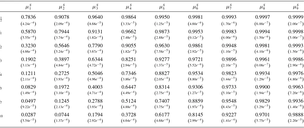
Table 2 contains the estimated unconditional probabilities πℓ,k for transitioning from absolute rating category ℓto
cate-gory k (this setsβℓk=0). While the probabilities in Table 1
are risk-neutral probabilities, the probabilities in this table are real-world probabilities. They represent the probability a firm currently in one ratings category will transition into another. From this matrix, we see that most transitions into default are coming from the lower rated categoriesℓ=1,2,3. The market does anticipate the defaults of many firms and market prices of traded assets (specifically CDS prices) do contain important information. Interestingly, we also find that transitions into de-fault do not monotonically decline as maturity increases. There is a reasonably large increase in the default probability for the best category ℓ=9. Some defaults appear to be a surprise to the market.
4.2 Comparison to Standard & Poors
In this section, we compare our ratings to those of Standard & Poors. Direct comparison of our ratings to S&P (or other agencies) is not obvious as they report 25 different letter grades from AAA to C as well as default. We map the letter grades into numeric grades.4First, we compare our ratings to S&P for those firms that defaulted. On the left ofFigure 2, we compare the average value of our ratings to S&P ratings as a function of the time until their default. The averages were taken for only
4The grades are mapped into numbers as AAA→25, AA+ →24, AA→23,
AA− →22, A+ →21, A→20, A− →19 BBB+ →18, BBB→17, BBB− →16, BB+ →15, BB→14, BB− →13, B+ →12, B→11, B− →10, CCC+ →9, CCC→8, CCC− →7, CC+ →6, CC→5, CC− →4, C+ →3, C→2, C→1, Default→0, Not Rated→ −1.
Table 2. Estimated unconditional matrix of transition probabilities
πℓ,k k=0 k=1 k=2 k=3 k=4 k=5 k=6 k=7 k=8 k=9
ℓ=0 1.0000 0.0000 0.0000 0.0000 0.0000 0.0000 0.0000 0.0000 0.0000 0.0000
ℓ=1 0.0060 0.8394 0.1077 0.0180 0.0085 0.0048 0.0039 0.0032 0.0026 0.0060
(0.0005) (0.0099) (0.0099) (0.0036) (0.0024) (0.0019) (0.0014) (0.0010) (0.0006) (0.0013)
ℓ=2 0.0048 0.0362 0.8988 0.0432 0.0028 0.0052 0.0025 0.0021 0.0017 0.0028
(0.0004) (0.0028) (0.0051) (0.0044) (0.0012) (0.0012) (0.0009) (0.0007) (0.0005) (0.0003)
ℓ=3 0.0015 0.0056 0.0122 0.9482 0.0272 0.0014 0.0008 0.0011 0.0007 0.0011
(0.0002) (0.0007) (0.0013) (0.0023) (0.0021) (0.0005) (0.0004) (0.0003) (0.0002) (0.0001)
ℓ=4 0.0003 0.0002 0.0008 0.0084 0.9743 0.0148 0.0004 0.0002 0.0002 0.0006
(0.0001) (0.0001) (0.0002) (0.0005) (0.0011) (0.0009) (0.0002) (0.0001) (0.0001) (0.0001)
ℓ=5 0.0001 0.0001 0.0001 0.0003 0.0092 0.9805 0.0090 0.0002 0.0001 0.0004 (9.2e−6) (2.1e−5) (2.9e−5) (6.5e−5) (0.0004) (0.0006) (0.0005) (0.0001) (4.8e−5) (3.4e−5) ℓ=6 0.0001 0.0001 0.0001 0.0001 0.0002 0.0081 0.9815 0.0096 0.0001 0.0001 (9.5e−6) (2.2e−5) (3.4e−5) (4.1e−5) (6.1e−5) (0.0003) (0.0005) (0.0004) (2.0e−5) (9.2e−6) ℓ=7 0.0000 0.0001 0.0001 0.0001 0.0001 0.0002 0.0088 0.9874 0.0030 0.0002 (9.8e−7) (9.6e−7) (2.1e−5) (3.1e−5) (3.9e−5) (6.1e−5) (0.0003) (0.0003) (0.0002) (1.6e−5)
ℓ=8 0.0002 0.0003 0.0003 0.0003 0.0002 0.0004 0.0004 0.0167 0.9793 0.0020
(0.00002) (0.0001) (0.0001) (0.0002) (0.0002) (0.0002) (0.0002) (0.0009) (0.0009) (0.0002)
ℓ=9 0.0018 0.0056 0.0028 0.0026 0.0053 0.0036 0.0072 0.0069 0.0174 0.9468
(0.0002) (0.0007) (0.0010) (0.0013) (0.0015) (0.0018) (0.0026) (0.0033) (0.0040) (0.0032)
NOTE: Posterior means and standard deviations of the transition probabilitiesπℓ,k,t=P(It=k|It−1=ℓ;Yit) assumingβℓ,k=0 of the mixture model forℓ=0, . . . , Ktok=0, . . . , K
withK=9. Categoryk=0 represents default, which is an absorbing state.
those firms that are rated by both us and S&P. We can see that on average our ratings lead the S&P ratings considerably, with the relative ratings providing the earliest signal of a firm’s distress. This graph corroborates the evidence fromTable 2, where most of the transitions into default come from firms in the lower ratings categories.
Next, we compare our ratings to S&P for those firms that we both rate and who did not default. This includes a total of 792 firms for the entire sample. On the right ofFigure 2, we compare the cumulative number of net ratings changes (sum of all past downgrades minus the sum of all past upgrades) through time of our absolute ratings to the S&P ratings. The vertical reference
line is the week of Lehman’s default in September 2008. For our ratings, the number of downgrades increases rapidly starting at the end of 2007 and continues to increase until the beginning of 2009. Conversely, the rate of change in S&P ratings only picks up months after Lehman’s default.
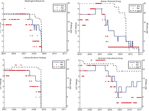
Figures3and4plot the absolute and relative ratings for eight different companies from January 2005 through February 2011. The new ratings (from k=0, . . . ,9) are labeled on the left-hand vertical axis in each plot. In the same graph, we also plot the Standard & Poors (S&P) rating for each of these firms on the right-hand vertical axis of each plot. By comparing the rel-ative ratings (red dashes) and absolute ratings (blue solid lines)
0 5 10 15 20 25
S&P Ratings
270 220 170 120 70 20 0
1 2 3 4 5 6 7 8 9
time until default measured in weeks
CGT Ratings
Mean Rating for Defaulted Firms Prior to Default
Abs Rel S&P
2006 2007 2008 2009 2010 2011 0
200 400 600 800 1000 1200
Cumulative Number of Net Ratings Changes (downgrades minus upgrades)
CGT absolute ratings S&P ratings
Figure 2. Left: Average rating across firms as a function of the time before default. Left vertical axis is our ratings scale and right vertical axis is S&P’s rating scale. Right: A comparison of the cumulative number of net ratings changes (downgrades minus upgrades) for our absolute ratings versus S&P ratings. The vertical reference line is the week of Lehman Brother’s default.
0
20050 2006 2007 2008 2009 2010 2011
1
20050 2006 2007 2008 2009 2010 2011
1
20050 2006 2007 2008 2009 2010 2011
1
20050 2006 2007 2008 2009 2010 2011
1
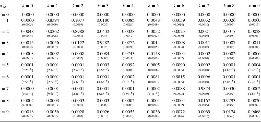
Figure 3. Absolute (bold line) and relative ratings (dotted line) for four firms from January 2005 through February 2011. Clockwise from the top left are AT&T, Zions Bancorporation, Autozone, and Yum! Brands. Left vertical axis is our ratings scale and right vertical axis is S&P’s rating scale.
for these companies, we can draw some interesting conclusions about the distribution of all companies’ ratings. Consider the case of YUM! Brands, AT&T, and Autozone inFigure 3. The absolute ratings for these companies remained roughly stable from 2005 through early 2011 but their relative ratings changed substantially. At the beginning of 2005, they were perceived as companies in the lower grade while by the end of the sample they are some of the better companies. S&P ratings are con-sidered to be relative ratings (i.e., they state that a firm rated AA is regarded as more creditworthy than a firm rated BB). Interestingly, while the market’s assessment of these firms rel-ative position changed, S&P ratings for both of these firms did not change as they remained rated BBB or BBB+ throughout 2005 to 2011. Finally, notice that the relative ratings change frequently because, by construction, they are not smoothed intertemporally.
Figure 4includes the relative, absolute, and S&P ratings of three financial firms Washington Mutual, Lehman Brothers, and Ambac Financial Group, which all defaulted over the course of the sample. In addition, we also plot the ratings of American International Group (AIG), which along with the first two firms
was at the center of the financial crisis. A striking feature of the ratings for these firms is that the relative ratings declined much faster than the absolute ratings. A comparison of the relative and absolute ratings provides a clear market signal of declining credit quality. Changes in these ratings can be observed in the data as early as the first quarter of 2007, whereas S&P did not substantially change the ratings until immediately prior to their default. Another striking difference in these plots is the ratings of Ambac Financial which had a relative rating equal to 1 for two years prior to finally defaulting. The new market implied ratings in many cases lead the downgrades by S&P by over a year.
Finally, output from the posterior distribution of the latent indicators p(I0:t|y1:t, D1:t;θ) can be used to construct credit
indicies for different sectors of the economy. Credit indices provide information to market participants, policy makers, and regulators about the state of the credit market. A simple index, which is easy to construct, is the percentage of firms in each absolute rating category through time. The upper left panel of Figure 5breaks the empirical distribution of the absolute ratings for all firms into five groups. We can see a dramatic decline in
0
20050 2006 2007 2008 2009 2010 2011
1
20050 2006 2007 2008 2009 2010 2011
1
20050 2006 2007 2008 2009 2010 2011
1
20050 2006 2007 2008 2009 2010 2011
1
Figure 4. Absolute (blue line) and relative ratings (red dotted line) for four firms from January 2005 through February 2011. Clockwise from the top left are Washington Mutual Inc., Ambac Financial, American International Group, and Lehman Brothers Inc. Left vertical axis is our ratings scale and right vertical axis is S&P’s rating scale.
the percentage of firms in the top tier (k=7,8,9) beginning in the middle of 2007. There is also a noticeable but more gradual increase in the percentage of firms in the lowest rated categories (k=0,1,2,3,4) peaking at the end of 2008.
The remaining plots ofFigure 5contain similar indices ex-cept that SIC industry codes are used to focus on subsectors of the economy. The top right graph includes the percentage of financial firms broken down into different categories. The plot illustrates that prior to 2007 most financial firms were well regarded by the market but this changed abruptly at the end of 2007 when financial markets recognized the impending crisis.
On the bottom left ofFigure 5, we plot similar percentages by absolute ratings category but only for deposit-taking financial institutions (commercial banks). We do the same for nondepos-itory credit/lenders in the bottom right-hand plot. Interestingly, we can see that prior to the end of 2007 almost all depository institutions were regarded as credit-worthy, mainly clustering into the top rated category (k=7,8,9), whereas the percentage of firms in these categories in March 2011 is almost zero. Credit indices like these provide a simple summary of debt markets and are a useful tool for regulators and policymakers who need to monitor the health of subsectors of the economy.
4.3 Loss distributions
The estimation of loss distributions for portfolios of bonds is an important ingredient in risk management. The past decade has seen a number of advancements in the modeling and estima-tion of default probabilities. Popular methods may focus only on defaults/bankruptcies, for example, Duffie, Saita, and Wang (2007), Koopman and Lucas (2008), and Duffie et al. (2009), or default data may be augmented with the addition of credit ratings transitions from Moody’s or Standard & Poors; for ex-ample, Gagliardini and Gouri´eroux (2005), Koopman, Lucas, and Monteiro (2008), Creal, Koopman, and Lucas (2013), and Creal et al. (2014). While it can be challenging to directly esti-mate models for large databases of CDS’s spreads or bonds, it is relatively easier to build models for thousands of firm’s credit ratings. As the market-based credit ratings discussed in this arti-cle are direct functions of asset prices, they can be incorporated into models for credit ratings transitions. Loss distributions for portfolios of bonds can then be constructed from credit rat-ings models. This provides a constructive and computationally tractable way to incorporate data from credit markets. It also leverages previous research on models for ratings transitions.
20050 2006 2007 2008 2009 2010 2011 0.1
0.2 0.3 0.4 0.5 0.6 0.7
Time
Percentage
Empirical distribution of absolute ratings
k = 0 + 1 + 2 + 3 + 4 k = 5
k = 6 k = 7 k = 8 + 9
20050 2006 2007 2008 2009 2010 2011 0.1
0.2 0.3 0.4 0.5 0.6 0.7 0.8 0.9 1
Empirical distribution of absolute ratings: Finance Industry
Time
Percentage
k = 0 + 1 + 2 + 3 + 4 k = 5
k = 6 k = 7 k = 8 + 9
20050 2006 2007 2008 2009 2010 2011 0.1
0.2 0.3 0.4 0.5 0.6 0.7 0.8 0.9 1
Time
Percentage
Percentage of firms by absolute ratings categories: Depository
k = 0 + 1 + 2 + 3 + 4 k = 5
k = 6 k = 7 + 8 + 9
20050 2006 2007 2008 2009 2010 2011 0.1
0.2 0.3 0.4 0.5 0.6 0.7 0.8 0.9 1
Time
Percentage
Percentage of firms by absolute ratings categories: Non−deposit credit
k = 0 + 1 + 2 + 3 + 4 k = 5
k = 6 k = 7 + 8 + 9
Figure 5. Each graph depicts the percentage of firms in different absolute ratings categories. Top left: All firms. Top right: All financial firms. Bottom left: All deposit-taking financial firms. Bottom right: All nondepository financial firms that are lenders.
We propose a simple alternative method for constructing loss distributions directly from the mixture model used for clus-tering. Consider a portfolio of companies for which we know the absolute ratings. As each rating category corresponds to a distribution over the space of risk-neutral survival functions, one can price a (hypothetical) 10-year zero-coupon, defaultable bond for each firm conditional on the current rating. This pro-vides an estimate of the current value of the portfolio. The loss distribution at any future horizon can then be viewed as a non-linear function of moments of the predictive distribution from the mixture model (1)–(3). Consistent with Bayesian inference for functions of the predictive distribution, we simulate future paths of the ratings forward through time for each company by iterating on the Markov transition matrix from the mixture model. For each simulated path of ratings, we simulate a se-quence of survival functions and compute a corresponding path of prices. These prices are then discounted back to the present using a discount factor curve constructed from the current Libor and interest rate swap prices. If a firm transitions into default, a
loss-given default is drawn by (statistically) bootstrapping from the empirical distribution of LGDs. The loss distributions are then built by comparing the current value of the portfolio to the value of the portfolio constructed from the simulated future paths of prices from the predictive distribution.
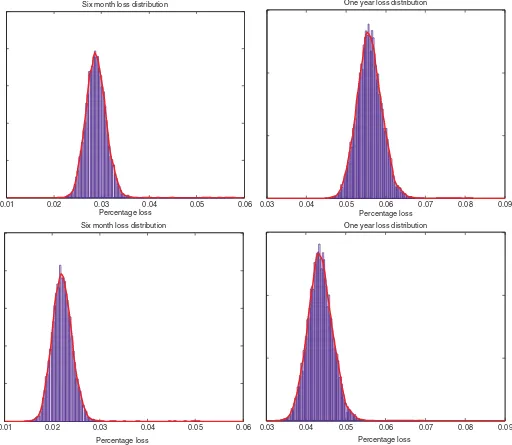
We illustrate this approach using the portfolio of 4461 rated companies on 2/23/2011. In practice, we do not condition on the current absolute rating but marginalize over the current ratings using the MCMC draws for the latent category indicators from the final time period{IT(j)}Mj=1.Figure 6contains the loss distribu-tions at the six-month (left column) and one-year (right column) horizons for two different discount rate curves that existed on 12/17/2008 and 2/23/2011. These are the top and bottom rows of Figure 6, respectively. Consistent with our expectations, the loss distributions during a period like the financial crisis (top row) are worse than a calmer period like early 2011. These graphs illustrate how the loss distributions are sensitive to interest rate variation or interest rate risk. An adverse movement in interest rates causes a rather substantial shift to the right in the loss
0.01 0.02 0.03 0.04 0.05 0.06 Percentage loss
Six month loss distribution
0.03 0.04 0.05 0.06 0.07 0.08 0.09
Percentage loss One year loss distribution
0.01 0.02 0.03 0.04 0.05 0.06
Percentage loss Six month loss distribution
0.03 0.04 0.05 0.06 0.07 0.08 0.09
Percentage loss One year loss distribution
Figure 6. Six-month (left) and one-year (right) loss distributions for a portfolio of 4461 companies rated at the end of the sample on 2/23/2011. The loss distributions were constructed using two different (risk-neutral) discount factor rate curves constructed from Libor and swap rates on 12/17/2008 (top row) and on 2/23/2011 (bottom row).
distribution for bonds. The loss distributions inFigure 6 condi-tion on a known discount rate curve, that is, the path of future (risk-free) discount rates are assumed to be known. By com-bining the market based ratings with a model for the future evolution of the discount rate curve (the term structure of inter-est rates), one can construct loss distributions that also reflect the uncertainty associated with future discount rates as well.
5. CONCLUSION AND DISCUSSION
We created new classes of credit ratings for publicly traded companies in the U.S. from actively traded assets. The new rat-ings include both absolute and relative ratrat-ings, which have dis-tinct economic interpretations. Our approach uses asset pricing data to impute a term structure of risk neutral survival functions or default probabilities. Firms are then clustered into ratings
cat-egories based on their survival functions using functional clas-sification. This allows all public firms whose assets are traded to be directly rated by market participants. Firms whose as-sets are not traded cannot be directly rated by the market but can be indirectly rated through the use of matching estimators. Our approach has the advantages of being timely (weekly data versus monthly or quarterly), simple to interpret economically, transparent, and computationally tractable. In addition, we have demonstrated that our ratings typically lead those of one of the major ratings agencies.
There are several extensions and further applications of the proposed model-based ratings. The standard matching estima-tor used here intentionally does not adjust for the presence of selection bias. Selection bias can occur if a firm is not traded for a reason that is unobservable to us and the imputed rating based on observable characteristics is not representative of its