Full Terms & Conditions of access and use can be found at
http://www.tandfonline.com/action/journalInformation?journalCode=ubes20
Download by: [Universitas Maritim Raja Ali Haji] Date: 11 January 2016, At: 22:49
Journal of Business & Economic Statistics
ISSN: 0735-0015 (Print) 1537-2707 (Online) Journal homepage: http://www.tandfonline.com/loi/ubes20
Further Results on the Limiting Distribution of
GMM Sample Moment Conditions
Nikolay Gospodinov , Raymond Kan & Cesare Robotti
To cite this article: Nikolay Gospodinov , Raymond Kan & Cesare Robotti (2012) Further
Results on the Limiting Distribution of GMM Sample Moment Conditions, Journal of Business & Economic Statistics, 30:4, 494-504, DOI: 10.1080/07350015.2012.694743
To link to this article: http://dx.doi.org/10.1080/07350015.2012.694743
Accepted author version posted online: 29 May 2012.
Submit your article to this journal
Article views: 479
Further Results on the Limiting Distribution
of GMM Sample Moment Conditions
Nikolay G
OSPODINOVDepartment of Economics, Concordia University, Montreal, Quebec, Canada H3G 1M8 ([email protected])
Raymond K
ANJoseph L. Rotman School of Management, University of Toronto, Toronto, Ontario, Canada M5S 3E6 ([email protected])
Cesare R
OBOTTIResearch Department, Federal Reserve Bank of Atlanta, Atlanta, GA 30309 ([email protected])
In this article, we examine the limiting behavior of generalized method of moments (GMM) sample moment conditions and point out an important discontinuity that arises in their asymptotic distribution. We show that the part of the scaled sample moment conditions that gives rise to degeneracy in the asymptotic normal distribution isT-consistent and has a nonstandard limiting distribution. We derive the appropriate asymptotic (weighted chi-squared) distribution when this degeneracy occurs and show how to conduct asymptotically valid statistical inference. We also propose a new rank test that provides guidance on which (standard or nonstandard) asymptotic framework should be used for inference. The finite-sample properties of the proposed asymptotic approximation are demonstrated using simulated data from some popular asset pricing models.
KEY WORDS: Asymptotic approximation; Generalized method of moments; Rank test;T-consistent estimator; Weighted chi-square distribution.
1. INTRODUCTION
Over the past 30 years, the generalized method of moments (GMM) has established itself as arguably the most popular method for estimating economic models defined by a set of moment conditions. In his seminal article, Hansen (1982) de-veloped the asymptotic distributions of the GMM estimator, sample moment conditions, and test of over-identifying restric-tions for possibly nonlinear models with sufficiently general dependence structure. This large sample theory proved to cover a large class of models and estimators that are of interest to researchers in economics and finance.
There are cases, however, in which the root-T convergence and asymptotic normality of the GMM sample moment condi-tions and estimators based on these moment condicondi-tions do not accurately characterize their limiting behavior. In particular, it is possible that some linear combinations of the GMM sample moment conditions have a degenerate distribution and the stan-dard limiting tools for inference are inappropriate. For example, Gospodinov, Kan, and Robotti (2010) demonstrated that some GMM estimators, which are functions of the sample moment conditions, are proportional to the GMM objective function and, hence, cannot be root-Tconsistent and asymptotically normally distributed for correctly specified models. This situation is di-rectly related to the results in lemma 4.1 and its subsequent discussion in Hansen (1982) that draw attention to the singular-ity of the covariance matrix of the sample moment conditions. However, to the best of our knowledge, the limiting behavior of the GMM sample moment conditions in the degenerate case, when the covariance matrix reduces to a matrix of zeros, has not been formally investigated in the literature.
In this article, we study some linear combinations of the sample moment conditions that give rise to degeneracy and an-alyze their asymptotic behavior. Interestingly, we show that in this case, the scaled sample moment conditions evaluated at the GMM estimator are characterized by a nonstandard limit-ing theory. More specifically, we demonstrate that the estimated GMM moment conditions converge to zero (the value implied by the population moment conditions) at rateT and have an asymptotic weighted chi-squared distribution. Besides being of academic interest, our results prove to be useful for inference in asset pricing models. Furthermore, a similar degeneracy oc-curs in the asymptotic analysis of Lagrange multipliers in the context of generalized empirical likelihood (GEL) estimation that has gained increased popularity in econometrics in recent years.
Nonstandard asymptotics (with an accelerated rate of con-vergence and nonnormal asymptotic distribution) often arises when the parameter of interest is near or on the boundary of the parameter space. Examples of this phenomenon include au-toregressive roots near or on the unit circle (Dickey and Fuller
1979; Phillips1987), (near) unit root in moving average models (Davis and Dunsmuir1996), local-to-zero signal-to-noise ra-tio in time-varying parameter models (Nyblom1989), and zero variance in nonnested model comparison tests (Vuong1989). In these cases, the rate of convergence of the estimated param-eter or test statistic of interest increases from root-T toT and
© 2012American Statistical Association Journal of Business & Economic Statistics
October 2012, Vol. 30, No. 4 DOI:10.1080/07350015.2012.694743
494
the asymptotic distribution changes from normal to a weighted chi-squared type of distribution. Interestingly, our article shows that similar nonstandard asymptotics can be encountered in seemingly regular GMM problems. It should also be noted that the degeneracy of the asymptotic distribution has been ana-lyzed in other contexts, although the existing results differ con-siderably from ours. See, for example, Sargan’s (1959,1983) discussion of nonlinear instrumental variable models with pos-sible singularity; Park and Phillips (1989) and Sims, Stock, and Watson (1990) for the analysis of time series models with a unit root; and Phillips (2007) for models with slowly varying regression functions.
The rest of this article is organized as follows. Section2 intro-duces the general setup and discusses an asset pricing example that illustrates the discontinuity in the asymptotic approximation of the sample moment conditions. This section also provides the main theoretical results on the limiting behavior of linear combinations of sample moment conditions and presents an easy-to-implement rank test that determines which asymptotic approximation should be used. Section3reports simulation re-sults based on a problem in empirical asset pricing and Section4
concludes.
2. ASYMPTOTICS FOR GMM SAMPLE MOMENT CONDITIONS
2.1 Notation and Analytical Framework
Letθ∈denote ap×1 parameter vector of interest with true value θ0 that lies in the interior of the parameter space andgt(θ) be a known function {g:Rp →Rm, m > p}of the data andθthat satisfies the set of population orthogonality conditions
E[gt(θ0)]=0m. (1) The GMM estimator ofθ0is defined as
ˆ
θ=arg minθ∈¯gT(θ)′WT¯gT(θ), (2) where WT is an m×m positive definite weight matrix and
¯gT(θ)=T1 T
t=1gt(θ).The matrixWT is allowed to be a fixed matrix that does not depend on the data and θ (the identity matrix, for example), a matrix that depends on the data but not onθ,or a matrix that depends on the data and a preliminary consistent estimator ofθ0as in the two-step and iterated GMM estimation. Given the first-order asymptotic equivalence of the two-step, iterated, and continuously updated GMM estimators, our subsequent results can be easily modified to accommodate the continuously updated (one-step) GMM estimator.
LetDT(θ)= T1 Tt=1 ∂gt(θ)
∂θ′ ,D(θ)=E ∂
gt(θ)
∂θ′
and make the following assumptions.
Assumption 1. Assume that
1
√
T
T
t=1
gt(θ0) d
→N(0m,V), (3)
whereV=∞
j=−∞E[gt(θ0)gt+j(θ0)′] is a finite positive def-inite matrix.
Assumption 2. Assume that
(a) gt(θ) is continuous in θ almost surely, E[supθ∈
|gt(θ)|]<∞,and the parameter spaceis a compact subset ofRp,
(b) there exists a uniqueθ0∈such thatE[gt(θ0)]=0m andE[gt(θ)]=0mfor allθ=θ0,
(c) WT p
→W,whereWis a nonstochastic symmetric posi-tive definite matrix,
(d) DT(θ) p
→D(θ) uniformly inθ on some neighborhood ofθ0andD0≡D(θ0) is of rankp.
Assumption 1 is a high-level assumption that implicitly im-poses restrictions on the data and the vectorgt(θ). The valid-ity of this assumption can either be verified in the particular context or it can be replaced by a set of explicit primitive con-ditions (see, for instance, Stock and Wright 2000). Assump-tion 2 imposes sufficient condiAssump-tions that ensureθˆ→p θ0in the interior of the compact parameter space.The uniform con-vergence and the full rank condition in Assumption 2 (d) are required for establishing the asymptotic distributions ofθˆand
¯gT(θˆ).
Under Assumptions 1 and 2,√T¯gT(θˆ) is asymptotically nor-mally distributed (Hansen1982, lemma 4.1) with mean zero and a singular asymptotic covariance matrix
0=[Im−D0(D′0WD0)−1D′0W]
×V[Im−D0(D′0WD0)−1D′0W]′. (4) Furthermore, it can be easily seen that the asymptotic covari-ance matrix of√TD′
0W¯gT(θˆ) reduces to ap×pmatrix of ze-ros that renders the asymptotic distribution of √TD′
0W¯gT(θˆ) degenerate. Provided that WT is a consistent estimator of
W, a similar degeneracy occurs for √TD′
0hT(θˆ), where
hT(θˆ)≡WT¯gT(θˆ).
It is interesting to note that this type of asymptotic degen-eracy extends to other setups and arises, for example, in the analysis of Lagrange multipliers in the GEL estimation of mo-ment condition models. In the GEL framework, the estimator of the Lagrange multipliers associated with the moment conditions takes a similar form ashT(θˆ) and has an asymptotic covariance matrix given byV−1
−V−1
D0(D′0V− 1
D0)−1D′0V− 1
(see, for in-stance, Smith1997). It is easy to see that premultiplying byD′
0 reduces this asymptotic variance to a zero matrix. Therefore, the results in this article can be adapted to deal with the possible asymptotic degeneracy of sample Lagrange multipliers in the GEL framework.
For our analysis, it is more convenient to rewrite the asymp-totic normality result in terms of the nonzero parts of the co-variance matrices of√T¯gT(θˆ) and
√
ThT(θˆ). LetQdenote an
m×(m−p) orthonormal matrix whose columns are orthogo-nal toW12D0. Then,
QQ′=Im−W 1 2D0(D′
0WD0)−1D′0W 1
2. (5)
Lemma 1. Under Assumptions 1 and 2,
√
TQ′W12¯gT(θˆ)→d N(0m
−p,Q′W 1 2VW
1
2Q) (6)
and
√
TQ′W−12hT(θˆ)→d N(0m−p,Q′W 1 2VW
1
2Q). (7) The role of matrixQin Lemma 1 is similar in spirit to the decomposition of Sowell (1996) in which themvector of nor-malized population moment conditionsW12E[gt(θ0)] is decom-posed intopidentifying restrictions used for the estimation ofθ that characterize the space of identifying restrictions andm−p
identifying restrictions that characterize the space of over-identifying restrictions. Lemma 1 shows that √TQ′W1
2¯gT(θˆ) and√TQ′W−1
2hT(θˆ) have a nondegenerate asymptotic normal distribution. However, little is known about the limiting behavior of those linear combinations of¯gT(θˆ) orhT(θˆ) that do not have an asymptotic normal distribution. The purpose of this article is to establish the rate of convergence and asymptotic distributions ofD′
0W¯gT(θˆ) andD′0hT(θˆ). Before we present our main result, we provide an example to illustrate the discontinuous nature of the asymptotic analysis for linear combinations of ¯gT(θˆ) or
hT(θˆ).
2.2 Motivation: An Asset Pricing Example
Letyt(θ) be a candidate stochastic discount factor (SDF) at timet, whereθis apvector of parameters of the SDF. Suppose we usemtest assets to estimate the true SDF parameter vector θ0as well as to test if the proposed SDF is correctly specified. Denote byRtthe payoffs of themtest assets at timetand byq the vector of the costs of themtest assets. Let
gt(θ)=Rtyt(θ)−q. (8) If the model is correctly specified, we haveE[gt(θ0)]=0m.A popular method of estimating θ0 is to choose θ to minimize the sample squared Hansen–Jagannathan (HJ, 1997) distance, defined as
ˆ
δ2T =min
θ ¯gT(
θ)′WT¯gT(θ), (9)
whereWT =
1 T
T t=1RtR′t
−1 .
To determine whether the proposed SDF is correctly specified, we can examine the sample pricing errors of themtest assets, that is, ¯gT(θˆ), where θˆ is the vector of estimated parameters chosen to minimize the sample HJ-distance. Alternatively, let λ denote an m×1 vector of Lagrange multipliers associated with the population moment conditions (pricing constraints) and consider the estimated Lagrange multipliers
ˆ
λ=WT¯gT(θˆ), (10) which are a transformation of the sample pricing errors. Hansen and Jagannathan (1997) showed that if the proposed SDF does not price the test assets correctly, then it is possible to correct the mispricing of the SDF by subtractingλ′Rt fromyt(θ). As a result, researchers are often interested in testingH0:λi =0, that is, in determining whether asset i is responsible for the proposed SDF to deviate from the true SDF.
Gospodinov, Kan, and Robotti (2010) showed that for a lin-ear SDF,q′λˆ = −δˆ2
T,where ˆδ 2
T =¯gT(θˆ)′WT¯gT(θˆ) is the squared sample HJ-distance. For the special case ofq=[1, 0′
m−1]′(i.e., the payoff of the first test asset is a gross return and the rest
are excess returns), the estimate of the Lagrange multiplier as-sociated with the first test asset, ˆλ1, isT-consistent and shares the weighted chi-squared distribution of ˆδ2
T under the assump-tion of a correctly specified model. This result is of practical importance since applied researchers often rely on the statisti-cal significance of individual Lagrange multipliers and pricing errors to determine whether an asset pricing model is correctly specified (Cochrane1996; Hodrick and Zhang 2001). Similar problems arise in other asset pricing contexts: for example, in conducting inference on the pricing errors associated with traded factors (see Pe˜naranda and Sentana2010). More generally, as we show below,
TD′0λˆ → −d (Ip⊗v′
2)v1, (11) wherev1andv2are jointly normally distributed vectors of ran-dom variables. As a result, any linear combination ofλˆ with a vector of weights that is in the span of the column space of
D0is alsoT-consistent with a nonstandard (product of normals) asymptotic distribution.
It is interesting to note that a similar type of discontinuity in the asymptotic approximation and accelerated rate of conver-gence have been established by Park and Phillips (1989) and Sims, Stock, and Watson (1990) in an AR(p) model,p >1, with a unit root in the AR polynomial. In particular, these arti-cles show that a linear combination ofWT¯gT(θ0) with a vector of weights [α1, . . . , αp]′=[ ¯α, . . . ,α¯]′,for some nonzero con-stant ¯α, is root-Tand asymptotically normally distributed, while a linear combination of WT¯gT(θ0) with a vector of weights [α1, . . . , αp]′=[ ¯α, . . . ,α¯]′ yields a T-consistent and asymp-totically nonnormally distributed estimator.
2.3 Main Results
We now turn to deriving the asymptotic distributions of
D′
0W¯gT(θˆ) andD′0hT(θˆ). Due to the similarities in their struc-ture, we first present the results for D′
0hT(θˆ) and discuss the case ofD′
0W¯gT(θˆ) in the next subsection. The following addi-tional assumption on the joint limiting behavior ofDˆT =DT(θˆ) andhT(θˆ) is needed to establish the asymptotic distribution of
D′
0hT(θˆ).
Assumption 3. Assume that
√
T
vec(Q′W1 2DˆT)
Q′W−12hT(θˆ)
d
→N 0(m−p)(p+1),
(12)
for some finite positive semidefinite matrix.
The asymptotic normality of them−pvectorQ′W−12hT(θˆ) follows directly from Lemma 1. The main requirement is on the limiting behavior of the matrixDˆT which is, however, rather weak and rules out only some trivial cases. It is important to note that we do not need to impose any restriction on the rate of convergence ofWT apart from being a consistent estima-tor of W (Assumption 2 (c)). In contrast, as we argue later, deriving the asymptotic distribution ofD′
0W¯gT(θˆ) requires ex-plicit assumptions on the rate of convergence ofWT that can differ for parametric and nonparametric heteroscedasticity and autocorrelation consistent (HAC) estimators.
We now state our main result in the following theorem.
Theorem 1. Under Assumptions 1–3,
TD′0hT(θˆ) d
→ −(Ip⊗v′2)v1, (13) wherev1andv2are (m−p)pand (m−p) vectors, respectively, and [v′
1, v′2]′∼N(0(m−p)(p+1),). Proof. See the Appendix.
To make the asymptotic approximation derived in Theo-rem 1 operational for conducting inference, we need an es-timate of the covariance matrix . In the following, we provide explicit expressions that can be used for consistent estimation of the covariance matrix in Theorem 1. Let
GT(θ)= T1tT=1∂vec(∂gt(θ)/∂θ′)/∂θ′, G(θ)=∂vec(D(θ))/
∂θ′, andG0≡G(θ0).
Assumption 4. Assume thatGT(θ) p
→G(θ) uniformly inθ on some neighborhood ofθ0,whereG(θ) exists, is finite, and is continuous inθ∈almost surely.
In the following lemma, we provide the explicit form of the matrix.
Lemma 2. LetG˜ =(Ip⊗Q′W 1
2)G0. Under Assumptions 1, 2, and 4, we have
=
∞
j=−∞
E[dtd′t+j], (14)
wheredt =[d′1,t, d′2,t]′and
d1,t = −G˜(D′0WD0)−1D′0Wgt(θ0)
+vec
Q′W12∂gt( θ0)
∂θ′
, (15)
d2,t =Q′W 1
2gt(θ0). (16)
Proof. See the Appendix.
The consistent estimation of the long-run covariance matrix can proceed by using a HAC estimator (see Andrews1991, for example) based on the sample counterparts ofd1,t andd2,t.
2.4 Discussion
The result in Theorem 1 has important implications for the asymptotic distribution of a linear combination ofhT(θˆ) with a weighting vectorαwhich is in the span of the column space of
D0. In particular, ifα=D0˜cfor a constant nonzeropvector˜c, then we have
Tα′hT(θˆ)→ −d ˜v′1v2, (17) where ˜v1 is the limit of
√
TQ′W12DˆT˜c, [˜v′
1, v′2]′∼
N(02(m−p),˜) with˜ =∞j=−∞E[˜dt˜d′t+j], ˜dt =[˜d′1,t, d′2,t]′ and ˜d1,t =(˜c′⊗Q′W
1 2)G0(D′
0WD0)−1D′0Wgt(θ0)+Q′W 1 2 ∂gt(θ0)
∂θ′ ˜c. Instead of expressing the asymptotic distribution as the inner product of two normal random vectors, the following
lemma shows that we can alternatively express it as a linear combination of independentχ2
1 random variables. Lemma 3. Suppose thatz=[z′
1, z′2]′, wherez1 andz2 are bothn×1 vectors, is multivariate normally distributed
z∼N(02n,), (18) whereis a positive semidefinite matrix with rankl≤2n. Let =SϒS′, whereϒis anl×ldiagonal matrix of the nonzero
eigenvalues ofandSis a 2n×lmatrix of the corresponding eigenvectors. In addition, let
Ŵ=ϒ12S′
⎡
⎢ ⎣
0n×n 1 2In 1
2In 0n×n ⎤
⎥ ⎦Sϒ
1
2. (19)
Then,
z′1z2∼ k
i=1
γixi, (20)
where theγi’s are thek≤lnonzero eigenvalues ofŴand the
xi’s are independentχ21random variables. Proof. See the Appendix.
This lemma shows that the inner product of two vectors of normal random variables (with mean zero) can always be written as a linear combination of independent chi-squared random vari-ables. This result proves very useful since it allows us to adopt numerical procedures for obtaining thep-value of a weighted chi-squared test that are already available in the literature (Imhof
1961; Davies1980; Lu and King2002). Furthermore, this result helps us to reconcile the form of the asymptotic approximation proposed in Theorem 1 with the weighted chi-squared distri-bution that arises in some special cases as in the asset pricing example.
Extending the result in Theorem 1 to cover the limiting behav-ior ofA′
0¯gT(θˆ),whereA0=WD0, requires stronger conditions. DefiningAˆT =WTDˆT, we need to replace Assumption 3 by as-suming
√
T
vec(Q′W−1 2AˆT)
Q′W1 2¯gT(θˆ)
d
→N 0(m−p)(p+1),
(21)
for some finite positive definite matrix. The conditions that (21) imposes on thempvector vec(AˆT −A0) can be best seen using the decomposition
√
T(AˆT −A0)=
√
T(WTDˆT−WD0)
=√TW(DˆT −D0)+
√
T(WT −W)D0
+√T(WT −W)(DˆT −D0)
=√TW(DˆT −D0)+
√
T(WT −W)D0
+op(1). (22) While the conditions for the matrixDˆT are easily satisfied (Assumption 3), the requirement of root-Tconvergence forWT rules out nonparametric HAC estimators (see Andrews 1991, for example) but allows for some parametric HAC estimators (West 1997). In general, this assumption requires that WT is
computed using a martingale difference sequence process or a dependent process for which the form of serial correlation is known. Then, under the assumption in (21), it can be shown, using similar arguments as in the proof of Theorem 1, that
TA′0¯gT(θˆ) d
→ −(Ip⊗u′2)u1, (23) where [u′
1, u′2]′∼N(0(m−p)(p+1),).We should note that, un-der some regularity conditions on the kernel function and band-width parameter as in Andrews (1991) and Hall and Inoue (2003), a similar limiting representation as in (23) can be de-rived for nonparametric HAC estimators but with a slower rate of convergence that depends on the smoothing parameter.
2.5 Rank Restriction Test
The speed of convergence ofα′hT( ˆθ) andα′W¯g
T(θˆ) depends crucially on whetherα is in the column span ofD0. In some cases, we know that α is in the column span of D0 (for in-stance, in our asset pricing example) and we should rely on the nonstandard asymptotics developed earlier to conduct statistical inference. In general, however, we do not know whetherα is in the column span of D0 and we need to resort to pretesting to determine which asymptotic framework should be used for the particular problem at hand. In the following, we propose a computationally attractive pretest that determines whetherαis in the span of the column space ofD0.
LetPαbe anm×(m−1) orthonormal matrix whose columns
are orthogonal toαsuch that
PαP′α=Im−α(α′α)−1α′. (24) Also, let=P′
αD0.It turns out that determining whetherαis in the span of the column space ofD0is equivalent to determining whetheris of reduced rank.
Under the null that is of (reduced) rank p−1, H0: rank()=p−1, there exists a nonzerop vector ˜c such that
D0˜c=α,or equivalently (by premultiplying byP′α and using
the properties ofPα)˜c=0m−1with the normalization˜c′˜c=1. As discussed in Cragg and Donald (1997), ifhas a reduced column rank ofp−1, we can use an alternative normalization and express one column of this matrix, sayπj,as a linear com-bination of the other columns, assuming that ˜cj =0.Without any loss of generality, we can order this column first and define the rearranged partitioned matrix=[π1, 2] such that
[π1, 2] ⎡
⎢ ⎢ ⎢ ⎢ ⎣
−1
c2 .. .
cp ⎤
⎥ ⎥ ⎥ ⎥ ⎦
=0m−1 (25)
or
2c0=π1, (26)
for some vector c0=[c2, . . . , cp]′. This is equivalent to im-posing a normalization on ˜csuch that its first element is−1. With such a normalization,c0is uniquely defined provided that rank()=p−1.
Let ˆT =P′
αDˆT. Using Assumption 3 and the proof of Lemma 2, it can be shown that
√
Tvec(ˆT −)→d N 0(m−1)p,M
, (27) whereM=∞
j=−∞E[m˜tm˜′t+j] and
˜
mt = −(Ip⊗P′α)G0(D′0WD0)−1D′0Wgt(θ0)
+vec
P′α
∂gt(θ0)
∂θ′
. (28)
In practice, M is replaced by a HAC estimator based on the sample counterparts of G0, D0, W, and gt(θ0). It should be stressed that the first term in the expression form˜t explicitly accounts for the estimation uncertainty inθˆ when gt(θ0) is a nonlinear function ofθ0. Whengt(θ0) is linear inθ0, the first term in the expression form˜t drops out (G0=0p×p) and the
second term does not depend onθ0. As a result, the asymptotic variance ofˆT depends only on the data and not onθ0.
LetlT(c)=ˆ2,Tc−πˆ1,T. Define the test statistic
LM=min
c T[lT(c)
′ˆT(c)−1lT(c)], (29)
where (c)=([−1, c′]⊗I
m−1)M([−1, c′]′⊗Im−1) and
ˆ
T(c) denotes its consistent estimator obtained by substituting a HAC estimator of M. The LM statistic tests the null hypothesis thatis of rankp−1 against the alternative that is of full rankp. The following lemma shows that the rank test statisticLMis chi-squared distributed withm−pdegrees of freedom under the null.
Lemma 4. Under Assumptions 1–4, andH0: rank()=p− 1,
LM→d χm2−p. (30) Proof See the Appendix.
It is important to note that the rank test statistic in Equation (29) is invariant to scaling ofc. Furthermore, we would like to emphasize that the minimization in (29) is with respect to only ap−1 vectorc, and the complexity of the minimization prob-lem does not increase withm. Although it can be shown (proof is available upon request) that theLM statistic in (29) is nu-merically equivalent to the test statistic proposed by Cragg and Donald (1997), it offers substantial computational advantages over the highly dimensional optimization problem in Cragg and Donald’s (1997) test. Finally, our simulation experiments show that the test in (30) enjoys excellent size and power properties.
3. ILLUSTRATION: LINEAR ASSET PRICING MODEL
In this section, we specialize our theoretical results to the linear specification of the asset pricing model in Section2.2and assess the accuracy of the proposed asymptotic approximation in this setup using a Monte Carlo simulation experiment. In particular, we evaluate the size of the weighted chi-squared test on the Lagrange multiplier associated with the first asset whenq=[1, 0′
m−1]′(i.e., the payoff of the first asset is a gross return and the payoffs of the other assets are excess returns). We consider two model specifications that are calibrated to monthly data for the period January 1932 to December 2006. The first
one is calibrated to the capital asset pricing model (CAPM) with the value-weighted market excess return as a risk factor. For the CAPM, the returns on the test assets are the gross return on the risk-free asset and the excess returns on 10 size ranked portfolios. The second specification is calibrated to the three-factor model (FF3) of Fama and French (1993) with risk factors given by the value-weighted market excess return, the return difference between portfolios of small and large stocks, and the return difference between portfolios of high and low book-to-market ratios. For FF3, the returns on the test assets are the gross return on the risk-free asset and the excess returns on 25 size and book-to-market ranked portfolios. All data are obtained from Kenneth French’s website. The SDFs of the CAPM and FF3 include an intercept term.
For each model, the factors and the returns on the test assets are drawn from a multivariate normal distribution. The covari-ance matrix of the factors and returns is chosen based on the covariance matrix estimated from the data. The mean return vec-tor is chosen such that the asset pricing model holds exactly for the test assets. For each simulated set of returns and factors, the unknown parametersθ0of the linear SDFyt(θ0)=˜ft′θ0, where
˜ft=[1, ft′]′withftdenoting the vector of risk factors, are esti-mated by minimizing the sample HJ-distance, which yields
ˆ
θ=(Dˆ′TWTDˆT)−1(Dˆ′TWTq), (31) whereDˆT = T1 Tt=1Rt˜ft′,WT =
1 T
T t=1RtR′t
−1
, andq=
[1, 0′
m−1]′. The estimated Lagrange multipliers are given by
ˆ
λ=WT¯gT(θˆ)=WT
1
T
T
t=1
Rtyt(θˆ)−q
, (32)
and we consider the first element ˆλ1. The next lemma special-izes the results in Theorem 1 and Lemma 2 to this setup. It should be noted that while Lemma 5 presents the limiting dis-tribution ofTλ1ˆ for the HJ-distance case, a similar result holds for any weighting matrixWT that converges in probability to a nonstochastic positive definite matrixW.
Lemma 5. Let D0=E[Rt˜ft′], V= ∞
j=−∞E[(Rt˜ft′θ0−
q)(Rt+j˜ft′+jθ0−q)′], W=(E[RtR′t])−1, Q denote an or-thonormal matrix whose columns are orthogonal toW12D0, and suppose that Assumptions 1–4 hold. Then,
Tλ1ˆ =Tq′λˆ → −d m−p
i=1
γixi, (33)
where thexi’s are independentχ21random variables and theγi’s are the eigenvalues of the matrixQ′W1
2VW− 1 2Q. Proof. See the Appendix.
In the analysis of the empirical size of our asymptotic approx-imation, the computedp-values from the weighted chi-squared distribution in (33) are compared to the 10%, 5%, and 1% the-oretical sizes of the test. For a comparison, we also provide the empirical size of a standard normal test ofH0:λ1 =0 used, for example, in Hodrick and Zhang (2001). The empirical rejec-tion probabilities are computed based on 100,000 Monte Carlo replications.
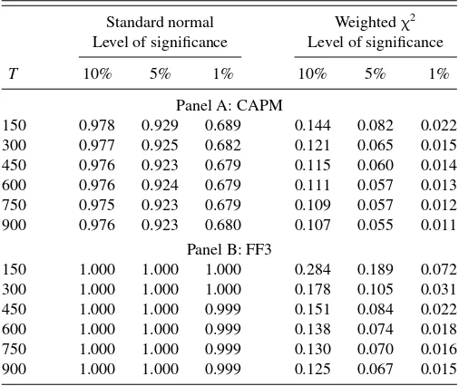
Table 1. Empirical sizes of the tests ofH0:λ1=0
Standard normal Weightedχ2
Level of significance Level of significance
T 10% 5% 1% 10% 5% 1%
Panel A: CAPM
150 0.978 0.929 0.689 0.144 0.082 0.022 300 0.977 0.925 0.682 0.121 0.065 0.015 450 0.976 0.923 0.679 0.115 0.060 0.014 600 0.976 0.924 0.679 0.111 0.057 0.013 750 0.975 0.923 0.679 0.109 0.057 0.012 900 0.976 0.923 0.680 0.107 0.055 0.011
Panel B: FF3
150 1.000 1.000 1.000 0.284 0.189 0.072 300 1.000 1.000 1.000 0.178 0.105 0.031 450 1.000 1.000 0.999 0.151 0.084 0.022 600 1.000 1.000 0.999 0.138 0.074 0.018 750 1.000 1.000 0.999 0.130 0.070 0.016 900 1.000 1.000 0.999 0.125 0.067 0.015
NOTE: The table presents the actual probabilities of rejection for the asymptotic tests of H0:λ1=0 with different levels of significance, assuming that the factors and returns are generated from a multivariate normal distribution. We consider two model specifications that are calibrated to monthly data for the period January 1932 to December 2006. The model specification in Panel A is calibrated to the capital asset pricing model (CAPM). The model specification in Panel B is calibrated to the three-factor model of Fama and French (FF3,1993). The results for different number of time series observations (T) are based on 100,000 simulations.
For different sample sizesT, we report the simulation results for the two model specifications in Panels A and B ofTable 1. In Panel A, the weighted chi-squared distribution provides a very accurate approximation to the finite-sample behavior of ˆλ1. In contrast, the standard normal test leads to severe size distortions and rejects the true null hypothesis about 92% of the time at the 5% significance level. In the case of 25 risky assets (Panel B), our approximation tends to overreject for small sample sizes. This overrejection is a well documented fact in empirical finance and occurs when the number of test assets mis large relative to the number of time series observationsT (see, for instance, Ahn and Gadarowski2004). AsTincreases, the empirical size of the weighted chi-squared approximation approaches its nominal level. In contrast, the standard normal test always rejects the true null hypothesis 100% of the time and does not improve as Tincreases.
While the incorrect size of the normal test is expected from our theoretical analysis, the severity of these size distortions is somewhat surprising and deserves further attention. Note that the conventionalt-statistic for testingH0:α′λ=0, whereα=
D0˜cand˜cis a nonzeropvector, is defined as
tα′λˆ =
√
Tα′λˆ
(α′WTˆWTα)12
= Tα
′λˆ
(Tα′WTˆWTα)12
, (34)
where ˆ denotes a consistent estimator of 0 in (4). Since
√
Tα′λˆ is asymptotically degenerate, it might be expected that
the t-test will be undersized, which stands in contrast to the overrejections reported in Table 1. The following lemma de-rives the asymptotic distribution of the t-statistic for testing
H0:α′λ=0 and shows that the numerator
√
Tα′λˆ and the
denominator [α′WTˆWTα]12 shrink to zero at the same rate, rendering the limit of the ratiotα′λˆ a bounded random variable.
Lemma 6. SupposeRt andftare iid multivariate elliptically distributed with finite fourth moments and kurtosis parameter
κ =µ4/(3σ4)−1, whereσ2andµ4are the second and fourth central moments of the elliptical distribution. LetH=E[˜ft˜ft′]+
κvar[˜ft]. Then,
tα′λˆ
d
→r√u+1−r2w, (35) wherer= −˜c′Hθ0/(˜c′H˜c)(θ′0Hθ0),u∼χ2
m−p, w∼N(0,1), anduandware independent of each other.
Proof. See the Appendix.
The result in Lemma 6 shows that the asymptotic distribution of the statistictα′λˆ is a mixture of two random variables. Also,
it is straightforward to show that the first and second moments of the asymptotic distribution in Lemma 6 are given by
E[tα′λˆ]=r
√
2Ŵ m−2p+1
Ŵ m−2p , (36)
whereŴ(·) is the gamma function, and
Etα2′λˆ=1+r2(m−p−1). (37) Whenα=q,we have that˜c=θ0,r= −1, and the test statis-tic ofH0:λ1=0 is asymptotically distributed as−
χ2m−p. One important implication of this result is that the correct asymptotic distribution of thet-statistic of ˆλ1is miscentered compared to the standard normal approximation and the shift to the left increases with the degree of overidentification. For example, the means of this limiting distribution for the CAPM (with m−p=9) and FF3 (withm−p=22) are−2.92 and−4.53, respectively. These results clearly illustrate that the standard asymptotic in-ference can be grossly misleading.
However, Lemma 6 also suggests that there are situations in which the standard normal distribution is still the appropriate limiting distribution oftα′λˆ. For example, this occurs whenr =0
or, equivalently, ˜c′Hθ
0=0. Since the mixing coefficient r is consistently estimable, the asymptotic approximation in Lemma 6 conveniently bridges these two extremes (r2=0 andr2=1). Next, we investigate the empirical size properties of the se-quential test of H0:α′λ=0 that uses the LM rank test of
H0: rank()=p−1 from Section2.5as a pretest. Recall that the rank test determines if the normal or the weightedχ2 distri-bution theory should be used for testing the hypothesis of interest
H0:α′λ=0.Table 2reports the empirical size and power of the reduced rank test whenαis in the span of the column space ofD0(α=q=[1, 0′m−1]′) or not (α=1m). Overall, the rank test exhibits excellent size and power properties.
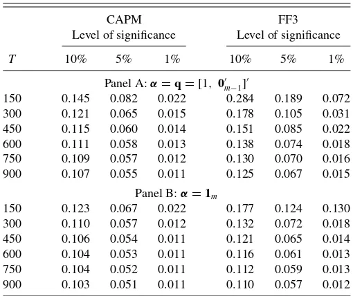
Table 3 presents the results on the empirical size of the
sequential test of H0:α′λ=0 for α=q=[1, 0′m−1]′ and α=1m by setting the nominal levels of the rank pretest and second-stage hypothesis test to be equal to each other. When α=q=[1, 0′
m−1]′,has a reduced rank and the second-stage test uses the weightedχ2
limiting distribution for inference. As a result, the size of the sequential test (Panel A inTable 3) is very similar to the size of the weightedχ2approximation reported in
Table 1. On the other hand, whenαis not in the column span
Table 2. Empirical size and power of the rank test
CAPM FF3
Level of significance Level of significance
T 10% 5% 1% 10% 5% 1%
Panel A:α=q=[1, 0′ m−1]′
150 0.095 0.044 0.007 0.069 0.024 0.001 300 0.098 0.048 0.009 0.093 0.044 0.007 450 0.099 0.050 0.009 0.098 0.047 0.008 600 0.099 0.049 0.010 0.099 0.047 0.009 750 0.100 0.050 0.010 0.100 0.049 0.009 900 0.099 0.050 0.010 0.100 0.050 0.009
Panel B:α=1m
150 0.999 0.997 0.965 0.977 0.913 0.531 300 1.000 1.000 1.000 1.000 1.000 1.000 450 1.000 1.000 1.000 1.000 1.000 1.000 600 1.000 1.000 1.000 1.000 1.000 1.000 750 1.000 1.000 1.000 1.000 1.000 1.000 900 1.000 1.000 1.000 1.000 1.000 1.000
NOTE: The table presents the actual probabilities of rejection for theLMrank test of H0: rank()=p−1 with different levels of significance, assuming that the factors and returns are generated from a multivariate normal distribution. We consider two model specifications (CAPM and FF3) that are calibrated to monthly data for the period January 1932 to December 2006. Panel A presents the empirical size of the rank test forα=q=
[1, 0′
m−1]′. Panel B reports the empirical power of the rank test forα=1m. The results for
different number of time series observations (T) are based on 100,000 simulations.
ofD0,the appropriate distribution theory is based on the con-ventional asymptotic normal approximation. Panel B inTable 3
reveals that in this case, the rank test successfully identifies the appropriate asymptotic framework and the empirical size of the sequential test is very close to its nominal level.
Table 3. Empirical size of the sequential test
CAPM FF3
Level of significance Level of significance
T 10% 5% 1% 10% 5% 1%
Panel A:α=q=[1, 0′ m−1]′
150 0.145 0.082 0.022 0.284 0.189 0.072 300 0.121 0.065 0.015 0.178 0.105 0.031 450 0.115 0.060 0.014 0.151 0.085 0.022 600 0.111 0.058 0.013 0.138 0.074 0.018 750 0.109 0.057 0.012 0.130 0.070 0.016 900 0.107 0.055 0.011 0.125 0.067 0.015
Panel B:α=1m
150 0.123 0.067 0.022 0.177 0.124 0.130 300 0.110 0.057 0.012 0.132 0.072 0.018 450 0.106 0.054 0.011 0.121 0.065 0.014 600 0.104 0.053 0.011 0.116 0.061 0.013 750 0.104 0.052 0.011 0.112 0.059 0.013 900 0.103 0.051 0.011 0.110 0.057 0.012
NOTE: The table presents the actual probabilities of rejection for the sequential test (which includes a reduced rank pretest) ofH0:λ1=0 with different levels of significance, assum-ing that the factors and returns are generated from a multivariate normal distribution. The nominal levels of the rank pretest and the second-stage test ofH0:λ1=0 are set equal to each other. We consider two model specifications (CAPM and FF3) that are calibrated to monthly data for the period January 1932 to December 2006. Panel A presents the empirical size of the sequential test forα=q=[1,0′
m−1]′, that is,αis in the span of the column space ofD0. Panel B reports the empirical size of the sequential test forα=1m, that is,α
is not in the span of the column space ofD0. The results for different number of time series observations (T) are based on 100,000 simulations.
4. CONCLUSION
This article derives some new results on the asymptotic dis-tribution of linear combinations of GMM sample moment con-ditions. These results complement lemma 4.1 of Hansen (1982) with the cases that give rise to singularity of the asymptotic covariance matrix and degeneracy of the asymptotic distribu-tion. Interestingly, we establish that in these cases, the GMM sample moment conditions converge at rateT to their popula-tion analogs and follow a nonstandard (weighted chi-squared) limiting distribution. Finally, we propose an easy-to-implement rank test to determine which asymptotic framework should be adopted for the particular problem at hand.
APPENDIX: PROOFS OF THEOREM AND LEMMAS
Proof of Theorem 1. Using the first-order condition
ˆ of normal random variablesv1.Similarly, using (7) in Lemma 1, let√TQ′W−1 This completes the proof of Theorem 1.
Proof of Lemma 2. To obtain the asymptotic distribution of vec(DˆT −D0), defineD˜T =T1
For the first term, we use the mean-value theorem to obtain
√ where the first equality follows from Assumption 4 and the second equality is ensured by the conditions imposed in As-sumption 2. For the second term, we have
√
2)G0. Stacking the expression for
√
This completes the proof of Lemma 2.
Proof of Lemma 3. Defining ˜z=S′z∼N(0
Sinceeis standard normal, it follows that
z′
xi’s are independentχ12 random variables. This completes the
proof of Lemma 3.
Proof of Lemma 4. Combining lT(c)=ˆ2,Tc−πˆ1,T = vec(ˆ2,Tc−πˆ1,T)=([−1, c′]⊗I
m−1)vec(ˆT) and Equation
(27), we have
be the estimator of c0. First, note that while the estimator ˆc depends on a preliminary estimatorθˆwhengt(θ) is a nonlinear function of θ, the uncertainty associated with the estimation of θ is already incorporated inM. Also, from the asymptotic equivalence of the estimator in (A.15) with the two-step GMM estimator, we have (Hansen1982)
√ Finally, using similar arguments as in Hansen (1982, lemma 4.2), it follows thatLMis asymptotically distributed as a chi-squared random variable with (m−1)−(p−1)=m−p de-grees of freedom. This completes the proof of Lemma 4.
Proof of Lemma 5. In the case of asset pricing models with a pricing constraint ¯gT(θ)=T1Tt=1Rtyt(θ)−q, the
ex-For the special case of a linear SDF that prices the test assets correctly, these expressions can be further simplified and have the form from the definition ofQ.
For the linear combinationTα′h
T(θˆ), where α=D0˜cand It is straightforward to show using the results above that
√
which is a linear combination of m−p independent chi-squared random variables with one degree of freedom. Since
v2∼N(0m−p,Q′W 1 2VW
1
2Q), the weights for the weighted
χ2 distribution are given by the eigenvalues of the matrix
Q′W12VW wherez1is the limiting distribution of
√ orthonormal matrix with its columns orthogonal toW
1 2 TDˆT. As a result, we can rewrite the term inside the squared root of the denominator of thet-statistic as
Tα′WTˆWTα=T˜c′D′0W
Conditional onz1, we have
z2∼N(21−111z1,22−21−11112). (A.32)
Noting thatQ′W1 pendent of each other. Then, we can write
tα′λˆ
If we assume that Rt and ft are iid multivariate ellipti-cally distributed, (A.34) can be greatly simplified. Suppose that (Xi, Xj, Xk, Xl) follow a multivariate elliptical distribution with multivariate kurtosis parameterκ. Using lemma 2 of Maruyama and Seo (2003), we have
ft are iid multivariate elliptically distributed, we can simplify the asymptotic distribution oftα′λˆ to
tα′λˆ random variable which is independent ofw. This completes the
proof of Lemma 6.
ACKNOWLEDGMENTS
We thank the Editor (Jonathan Wright), an Associate Ed-itor, two anonymous referees, Marine Carrasco, Francisco Pe˜naranda, Peter Phillips, Enrique Sentana, Chu Zhang and the seminar participants at Columbia University and the Uni-versity of British Columbia for helpful comments and sugges-tions. Gospodinov gratefully acknowledges financial support from Fonds de recherche sur la soci´et´e et la culture (FQRSC), Institut de finance math´ematique de Montr´eal (IFM2), and the Social Sciences and Humanities Research Council of Canada. Kan gratefully acknowledges financial support from the Na-tional Bank Financial of Canada and the Social Sciences and Humanities Research Council of Canada. The views expressed here are those of the authors’ and not necessarily those of the Federal Reserve Bank of Atlanta or the Federal Reserve System.
[Received August 2011. Revised May 2012.]
REFERENCES
Ahn, S. C., and Gadarowski, C. (2004), “Small Sample Properties of the GMM Specification Test Based on the Hansen-Jagannathan Distance,”Journal of Empirical Finance, 11, 109–132. [499]
Andrews, D. W. K. (1991), “Heteroskedasticity and Autocorrelation Consistent Covariance Matrix Estimation,”Econometrica, 59, 817–858. [497,498] Cochrane, J. H. (1996), “A Cross-Sectional Test of an Investment-Based Asset
Pricing Model,”Journal of Political Economy, 104, 572–621. [496] Cragg, J. G., and Donald, S. G. (1997), “Inferring the Rank of a Matrix,”Journal
of Econometrics, 76, 223–250. [498]
Davies, R. B. (1980), “Algorithm AS 155: The Distribution of a Linear Combi-nation ofχ2Random Variables,”Applied Statistics, 29, 323–333. [497] Davis, R. A., and Dunsmuir, W. T. M. (1996), “Maximum Likelihood Estimation
for MA(1) Processes With a Root on or Near the Unit Circle,”Econometric Theory, 12, 1–29. [494]
Dickey, D. A., and Fuller, W. A. (1979), “Distribution of the Estimators for Autoregressive Time Series With a Unit Root,”Journal of the American Statistical Association, 74, 427–431. [494]
Fama, E. F., and French, K. R. (1993), “Common Risk Factors in the Returns on Stocks and Bonds,”Journal of Financial Economics, 33, 3–56. [499] Gospodinov, N., Kan, R., and Robotti, C. (2010), “On the Hansen-Jagannathan
Distance With a No-Arbitrage Constraint,” Working Paper, Federal Reserve Bank of Atlanta. [494,496]
Hall, A. R., and Inoue, A. (2003), “The Large Sample Behaviour of the Gener-alized Method of Moments Estimator in Misspecified Models,”Journal of Econometrics, 114, 361–394. [498]
Hansen, L. P. (1982), “Large Sample Properties of Generalized Method of Moments Estimators,”Econometrica, 50, 1029–1054. [494,495,501,502] Hansen, L. P., and Jagannathan, R. (1997), “Assessing Specification
Er-rors in Stochastic Discount Factor Models,” Journal of Finance, 52, 557–590. [496]
Hodrick, R., and Zhang, X. (2001), “Evaluating the Specification Errors of Asset Pricing Models,”Journal of Financial Economics, 62, 327–376. [496,499] Imhof, J. P. (1961), “Computing the Distribution of Quadratic Forms in Normal
Variables,”Biometrika, 48, 419–426. [497]
Lu, Z. H., and King, M. L. (2002), “Improving the Numerical Technique for Computing the Accumulated Distribution of a Quadratic Form in Normal Variables,”Econometric Reviews, 21, 149–165. [497]
Maruyama, Y., and Seo, T. (2003), “Estimation of Moment Parameters in El-liptical Distributions,”Journal of Japan Statistical Society, 33, 215–229. [503]
Nyblom, J. (1989), “Testing for the Constancy of Parameters Over Time,” Journal of the American Statistical Association, 84, 223–230. [494] Park, J. Y., and Phillips, P. C. B. (1989), “Statistical Inference in
Regres-sions With Integrated Processes: Part 2,”Econometric Theory, 5, 95–131. [495,496]
Pe˜naranda, F., and Sentana, E. (2010), “A Unifying Approach to the Empirical Evaluation of Asset Pricing Models,” Working Paper, Universitat Pompeu Fabra. [496]
Phillips, P. C. B. (1987), “Towards a Unified Asymptotic Theory for Autore-gression,”Biometrika, 74, 535–547. [494]
——— (2007), “Regression With Slowly Varying Regressors and Nonlinear Trends,”Econometric Theory, 23, 557–614. [495]
Sargan, J. D. (1959), “The Estimation of Relationships With Autocorrelated Residuals by the Use of Instrumental Variables,”Journal of the Royal Sta-tistical Society,Series B, 21, 91–105. [495]
——— (1983), “Identification and Lack of Identification,”Econometrica, 51, 1605–1633. [495]
Sims, C. A., Stock, J. H., and Watson, M. W. (1990), “Inference in Linear Time Series Models With Some Unit Roots,” Econometrica, 58, 113– 144. [495,496]
Smith, R. J. (1997), “Alternative Semi-Parametric Likelihood Approaches to Generalized Method of Moments Estimation,”Economic Journal, 107, 503– 519. [495]
Sowell, F. B. (1996), “Optimal Tests for Parameter Instability in the Generalized Method of Moments Framework,”Econometrica, 64, 1085–1107. [496] Stock, J. H., and Wright, J. H. (2000), “GMM With Weak Identification,”
Econometrica, 68, 1055–1096. [495]
Vuong, Q. H. (1989), “Likelihood Ratio Tests for Model Selection and Non-Nested Hypotheses,”Econometrica, 57, 307–333. [494]
West, K. D. (1997), “Another Heteroskedasticity and Autocorrelation Con-sistent Covariance Matrix Estimator,” Journal of Econometrics, 76, 171–191. [497]