On Connecting Orbits of
Semilinear Parabolic Equations on
S
1Yasuhito Miyamoto
Received: August 3, 2003 Revised: June 30, 2004
Communicated by Bernold Fiedler
Abstract. It is well-known that any bounded orbit of semilinear parabolic equations of the form
ut=uxx+f(u, ux), x∈S1=R/Z, t >0,
converges to steady states or rotating waves (non-constant solutions of the formU(x−ct)) under suitable conditions onf. Let S be the set of steady states and rotating waves (up to shift). Introducing new concepts — the clusters and the structure of S —, we clarify, to a large extent, the heteroclinic connections within S; that is, we study which u ∈ S and v ∈ S are connected heteroclinically and which are not, under various conditions. We also show that ♯S ≥ N+PNj=1[[
p
(fu(rj,0))+/(2π)]] where{rj}Nj=1is the set of the roots
off(·,0) and [[y]] denotes the largest integer that is strictly smaller than y. In paticular, if the above equality holds or if f depends only on u, thestructureof S completely determines the heteroclinic connections.
2000 Mathematics Subject Classification: 35B41, 34C29
Keywords and Phrases: global attractor, heteroclinic orbit, zero num-ber, semilinear parabolic equation.
Contents
1. Introduction 436
2. Notation and Main Theorems 438
3. Proof of the Key Lemma 447
4. Preparation for the Proof of Theorem A 455
6. Proof of Theorems A and C 459
7. Proof of Theorem A’ and Lemma F’ 463
8. Proof of Proposition D 465
References 467
1. Introduction
We will investigate the global dynamics of semilinear parabolic partial dif-ferential equations onS1=R/ZinX =C1(S1)
(1.1)
(
ut=uxx+f(u, ux), x∈S1,
u(x,0) =u0(x), x∈S1.
The above problem is equivalent to a problem on the interval [0,1] under the periodic boundary conditions u(0, t) = u(1, t), ux(0, t) = ux(1, t) for t > 0.
Under suitable conditions on f, the solutions of (1.1) exist globally int > 0. Thus (1.1) defines a global semiflow Φt on X. We will call each solution of
(1.1) an orbit.
Angenent and Fiedler [AF88] and Matano [Ma88] have shown independently that any solution of (1.1) approaches as t → ∞ to a solution (or a family of solutions) of the formU(x−ct), wherecis some real constant. SinceU(x−ct) is a solution to (1.1), the functionU(ζ) should satisfy the following equation:
(1.2) d
2U
dζ2 +c
dU dζ +f
µ
U,dU dζ
= 0, ζ∈S1,
whereζ=x−ct. Note thatU(ζ+θ) is a solution to (1.2) for allθ∈S1provided
that U(ζ) is a solution. If c6= 0 and if U(ζ) is not a constant function, then U(x−ct) is a time periodic solution called a rotating wave with speed c. If c = 0 and if U(ζ) is not a constant function, then U(x) is called a standing wave. Thus steady states consist of both standing waves and constant steady states. By using these terms, the above assertion can be restated that any solution of (1.1) approaches either rotating waves or steady states.
Under suitable conditions onf that will be specified later, (1.1) has the set A ⊂X called the global attractor. This setAis characterized as the maximal compact invariant set and it attracts all the orbits of (1.1).
Matano and Nakamura [MN97] have shown that the global attractor A of (1.1) consists of rotating waves, standing waves andconnecting orbitsthat con-nect these waves. Therefore, in order to understand the dynamical structure of A it is important to know which pairs of waves are connected heteroclini-cally and which pairs are not. The paper [AF88] proves the existence of some connecting orbits for the problem (1.1) by using a topological method. We are interested in finding out a sharper criterion for the existence of connecting orbits.
every wave is odd or zero, then certain order relations among waves defined below and the Morse index of all the waves determine which pairs of waves are connected heteroclinically and which pairs are not (Theorem A). In particular, if the actual number of the waves coincides with the lower bound given in Corollary B, then the hypothesis of Theorem A is automatically fulfilled, hence the heteroclinic connections are completely determined (Theorem C). In the special case where f depends only on u, we can completely determine which pairs of waves are connected heteroclinically and which are not (Theorems A and A’), and we will present rather simple and explicit sufficient conditions on f for the hypotheses of Theorem C to be satisfied (Proposition D).
Theorems A and C and Proposition D are proved by using the concepts of
clusters and the structurewhich we introduce in Section 2. Let S be the set of all the waves. Roughly speaking, a cluster is a subset of S consisting of waves sharing certain common features, andS is expressed as a disjoint union ofclusters. One can show that eachclusteris a totally ordered set with respect to the following order relation
u⊲v ⇐⇒def R(u)⊃R(v),
where R(u) denotes the range of u (see Definition 2.5 and Remark 2.6). We then define thestructureofS by associating eachclusterwith the sequence of (modified) Morse indices of its elements. Lemmas E, F and F’ give fundamental properties of this sequence of modified Morse indices.
Now, many authors study the global attractor of (1.1) for the case where the boundary conditions in (1.1) is replaced by the Dirichlet or the Neumann boundary conditions. We can see [BF89] for the Dirichlet boundary conditions, [FR96] and [Wo02] for the Neumann boundary conditions and [MN97] for pe-riodic boundary conditions. Here we recall the results of [FR96]. In the case of the Neumann boundary conditions on [0,1], the global attractor consists of the steady states and the connecting orbits between these steady states, if all the steady states are hyperbolic. Let {Uj(x)}nj=1 (U1(0) < U2(0)<· · · < Un(0))
be the set of all the steady states. Roughly speaking, the permutation that re-arranges the sequence (U1(1), U2(1), . . . , Un(1)) in increasing order determines
the Morse indices of all the steady states and the zero number of functions Uj(x)−Uk(x) (1≤j < k≤n) (In brief, the zero number of a function, which
is defined in Section 2, is the number of the roots of the function). Once these Morse indices and the zero number of the difference of all the pairs among the waves are obtained, then this information tells which steady states are con-nected and which are not. Wolfrum [Wo02] has simplified the conditions of whether steady states are connected heteroclinically or not using the concept ofk-adjacent. The concept ofk-adjacentalso uses the zero number of functions Uj(x)−Uk(x) and the value of one of end points Uj(0) (or Uj(1)). In the
the waves play an important role in determining the Morse index of the waves and the zero number of the difference of the pairs, thereby giving the global picture of their heteroclinic connection.
This paper is organized as follows: In Section 2 we introduce some notation and definitions and state our main results (Theorems A A’ and C, Corollary B, Proposition D and Lemmas E, F and F’). Roughly speaking, Corollary B gives a lower bound for the number of the waves in terms of the derivatives of f, and Lemma F is concerned with the modified Morse indices of waves and the structure ofclusters. Theorems A, A’ and C and Proposition D determine the heteroclinic connections among waves under various conditions. In Section 3 we will prove Lemma 3.1 which is the key lemma of this paper. In Section 4 we will show that each clusteris a totally ordered set in our order relation. We state the main results of [AF88]. We will prove Theorem C by using the results. In Section 5 we will investigate a sequence of modified Morse indices of waves in eachclusterand prove Lemmas E and F and Corollary B. In Section 6 we will prove Theorem A, using Lemma F and main results of [AF88]. In Section 7 we consider the case where f depends only on u. We will prove Theorem A’ and Lemma F’. In Section 8 we prove Proposition D, which is a special case of Theorems A and A’. We will give rather simple and explicit sufficient conditions onf under which all theclustersaremonotoneandsimple, the meaning of which will be defined in Section 2. The monotonicity and
simplicityofclustersautomatically determine the Morse index of all the waves and the zero number of the difference of the pairs among the waves, hence their heteroclinic connections.
Acknowledgment. The author would like to thank Professor H. Matano for his valuable comments and many fruitful discussions, and thank the referee for his/her useful suggestions. He would also like to express his gratitude to Professor B. Fiedler, whose early work has given the author much inspiration.
2. Notation and Main Theorems
In this paper the nonlinear termf satisfies the following assumptions:
(A1) f:R×R→Ris a C3-function.
(A2) There exists a constant L1 >0 such thatu·f(u,0)<0 for |u|> L1, and the function f(·,0) has finitely many real roots.
(A3) ( i ) For any solutionu(x, t) to (1.1), ||u(·, t)||C1
(S1
) := ||u(·, t)||C0
(S1
) + ||ux(·, t)||C0
(S1
) remains
bounded ast→ ∞.
(ii) There exists a constantL2>0 such that
||U(ζ)||C1(
R):=||U(ζ)||C0(
for any periodic solution or constant solutionU(ζ) to the following equation:
(2.1) d
2U
dζ2 +c
dU dζ +f
µ
U,dU dζ
= 0, ζ∈R,
wherecis an arbitrary real number.
The assumption (A3) (ii) will be needed in Section 3, where we study the bifu-cation structure of rotating waves and constant steady states. The assumption (A3) is satisfied if the following condition (A3)′ holds:
(A3)′ For any constant M1 > 0, there exists a constant L3 > 0 such that fu(u, p)≤0 for|u|< M1 and|p|> L3.
From (A1), (A2) and (A3) it follows that (1.1) defines a global semiflowΦt
onX that is dissipative. Here a semiflowΦt onX is called dissipativeif there
exists a ballB⊂X which satisfies the following: For anyu0∈X, there exists
t0>0 such thatΦt(u0)∈B for allt≥t0(see [Ma76]).
Hereafter, we assume (A1)+(A2)+(A3)′ throughout the present paper.
By the standard parabolic estimates, the mappingΦtis a compact mapping
for everyt >0. This, together with the dissipativity of Φt, implies that there
is the (nonempty) maximal compact invariant set A ⊂ X. It is well-known from the general theory of dissipative dynamical systems that Ais connected and attracts all the orbits of (1.1). This set Ais called the global attractor. The Hausdorff dimension ofAof (1.1) is 2 [M/2] + 1 whereM is the maximal generalized Morse index of the steady states or the rotating waves (see [MN97]). Let us introduce some definitions and notation. In this paper we denote by S the set of steady states and rotating waves of (1.1). Note that ifU(x−ct) is a rotating wave (or a steady state in the case wherec= 0), thenU(x−ct+θ) is also a rotating wave (or a steady state) for anyθ∈S1. Hereafter we identify
U(·) and U(· +θ). In other words, we will understand S to be the set of equivalence classes, each of which is expressed in the form
Γ(U) :={U(x−ct+θ)|θ∈S1},
where U(ζ) is a solution of (1.2). However in order to simplify notation, we write U(x−ct)∈ S to mean [U(x−ct)]∈ S, where [U(x−ct)] denotes the equivalence class to whichU(x−ct) belongs. Thereforeu(x, t)∈S shall mean that u(x, t) =U(x−ct+θ) for someθ∈S1 whereU(ζ) is a solution to (1.2).
Furthermore, by a heteroclinic connection from u(x, t)(:= U(x−ct)) ∈ S to v(x, t)(:= V(x−˜ct))∈S we mean that there is an orbitw(x, t) of (1.1) such that
inf
θ1∈S1
kw(x, t)−U(x−ct+θ1)kL∞
(S1)→0 (t→ −∞),
inf
θ2∈S1
In particular, if U andV are ‘hyperbolic’ (whose meaning is defined below in this section), then a heteroclinic connection fromuto vautomatically implies the following stronger convergence:
kw(x, t)−U(x−ct+θ1)kL∞
(S1
)→0 (t→ −∞) for someθ1∈S1,
kw(x, t)−V(x−˜ct+θ2)kL∞
(S1
)→0 (t→+∞) for someθ2∈S1.
The number of the roots of f(·,0) is finite owing to (A2). Let {rj}Nj=1
(r1< r2<· · ·< rN) be the roots off(·,0) throughout the present paper. All
the constant steady states are u(x, t) =rj (j∈ {1,2, . . . , N}).
Remark 2.1. Iffu(rj,0)6= 0 for allj∈ {1,2, . . . , N}, thenN is odd because of
(A2). Moreover u(x, t) =rj (j ∈ {1,3,5, . . . , N}) is a stable constant steady
state, whileu(x, t) =rj(j∈ {2,4,6, . . . , N−1}) is an unstable constant steady
state (see Remark 2.8 below).
The zero number is a powerful tool to analyze nonlinear single reaction-diffusion equations in one space dimension:
z(w) :=♯©
x|w(x) = 0, x∈S1ª
forw∈X,
where ♯Y denotes the number of elements of the set Y. It is well-known that z(w(·, t)) is a non-increasing function oftifwis a solution of a one-dimensional linear parabolic equation (see [Ma82], [Ni62] and [St36]). Furthermore, the following proposition holds:
Proposition 2.2 (Angenent and Fiedler [AF88] and Angenent [An88]). Let
a(x, t)andb(x, t)beC2-functions in(x, t)∈S1×(0, τ) (τ >0). Letw(x, t)∈X
be a solution to the following equations:
wt=wxx+a(x, t)wx+b(x, t)w, (x, t)∈S1×(0, τ).
Thenz(w(·, t))is finite for every t∈(0, τ)and is non-increasing int. More-over z(w(·, t)) drops at each t = t0 when the function x 7−→ w(x, t0) has a
multiple zero.
Remark 2.3. Angenent and Fiedler [AF88] have proved Proposition 2.2 in the case wherea(x, t) andb(x, t) are real analytic functions. Angenent [An88] has relaxed this analyticity assumption.
Using the moving frame with speedc, we can rewrite (1.1) as follows: (2.2) ut=uζζ+cuζ +f(u, uζ),
whereζ=x−ct. LetU(x−ct)∈S. The waveU(ζ)(=U(x−ct)) is a steady state of (2.2). In order to analyze the stability ofU(ζ), we define the linearized operator of (2.2) atU(ζ) by
LUw=wζζ+cwζ+fu(U, Uζ)w+fp(U, Uζ)wζ, ζ∈S
1,
provided that U is a non-constant steady state of (2.2). Here fp denotes the
derivative of f with respect to the second variable. IfU is a constant steady state of (2.2), then we define the linearized operator by
LUw=wζζ+fu(U,0)w+fp(U,0)wζ, ζ∈S
By the standard spectral theory for ordinary differential operators of the second order, the spectrum ofLU consists of eigenvalues of finite multiplicity and has no accumulation point except ∞. Let{λn}∞n=0 be the eigenvalues ofLU that are repeated according to their algebraic multiplicity. We define the Morse index of U ∈ S by i(U) := ♯{λn| Re(λn) > 0}. By a Sturm-Liouville type
theorem (see [AF88] and [MN97]), we have
Re(λ0)>Re(λ1)≥Re(λ2)>Re(λ3)≥ · · · ≥Re(λ2j)>Re(λ2j+1)≥ · · ·.
Moreover if U is a non-constant steady state, we can see (2.3) i(U)∈ {z(Uζ), z(Uζ)−1}
(see [AF88] and [MN97]). Note thatz(Uζ) is even andz(Uζ)−1 is odd sinceUζ
is a periodic function ofζ. We can see the Morse index of the constant steady states by easy calculations (see Remark 2.8 below).
Next we define the hyperbolicity of U ∈S. Because of translation equivari-ance of the equation (1.1), each rotating wave and each non-constant steady state form a one-dimensional manifold that is homeomorphic toS1. This
equiv-ariance has to be taken into account when we define the hyperbolicity of those solutions.
Definition 2.4.
( i ) Let u be a (non-constant) rotating wave (c 6= 0) or a non-constant steady state(c= 0). We sayuis hyperbolic if0 is the only eigenvalue of Lu on the imaginary axis and if0 is a simple eigenvalue.
(ii) Let ube a constant steady state(i.e. u(x, t) =rj). We sayuis
hyper-bolic if there is no eigenvalue ofLu on the imaginary axis. Definition 2.5. Let u(x, t)be a solution of(1.1). We define
R(u(·, t)) :=
½
y∈R
¯ ¯ ¯ ¯
min
x∈S1u(x, t)≤y≤maxx∈S1u(x, t)
¾
.
Remark 2.6. Ifu∈S, thenR(u(·, t)) is independent oft. Hereafter we simply writeR(u) ifu∈S.
Definition 2.7. Foru∈S, we define its “modified Morse index” by
I(u) :=
z(ux) if u is not a constant steady state;
i(u) + 1 if u is an unstable constant steady state; 0 if u is a stable constant steady state.
Remark 2.8. One can calculate the Morse index of the constant steady states. Letube a constant steady state (i.e. u(x) =rj). Then
i(u) =
2
" p
fu(rj,0)
2π
#
+ 1 if fu(rj,0)>0;
where [y] denotes the largest integer not exceedingy. If all the constant steady states are hyperbolic, theni(u) = 2[p
fu(rj,0)/(2π)]+1 forj∈ {2,4,6, . . . , N−
1}andi(u) = 0 forj∈ {1,3,5, . . . , N}. Thusrj (j∈ {1,3,5, . . . , N}) is stable
andrj (j∈ {2,4,6, . . . , N−1}) is unstable.
Note that I(u) is always a non-negative even integer. From (2.3) it follows that
i(u)≤I(u)≤i(u) + 1.
ThereforeI(u) is a good approximation of the real Morse index i(u). Clearly, I(u) =i(u) if and only ifi(u) is even.
While the modified Morse indexI(u) is easily computable from Definition 2.7 and Remark 2.8, the real Morse index i(u) is not always easily to determine. This is the reason why we introduce the notion modified Morse index.
Now we can define thecluster.
Definition 2.9. Let 1≤k≤l≤N. We define the clusters by
Ckl:={u∈S| Skl⊂R(u), ({r1, r2, . . . , rN}\Skl)∩R(u) =∅},
whereSkl:={rk, rk+1, . . . , rl}.
It is not difficult to see that
Ckl∩Ck′l′ =∅ if (k, l)6= (k′, l′),
S= [
1≤k≤l≤N
Ckl.
Furthermore one can see that, ifkor lis odd, then Ckk={rk} and Ckl=∅ (k6=l).
The concept ofclusterswill be useful in the phase plane analysis as we will see in Section 6.
Definition 2.10. LetCkl be a cluster. We define
R(Ckl) := [
u∈Ckl R(u).
Definition 2.11. Letu, v ∈S. We define the order relation ofS as follows:
u⊲v ⇐⇒def R(u)⊃R(v).
Letu, v, w∈S. Ifu⊲v, then we sayv is smaller thanuin the order⊲, and
uis bigger than v in the order⊲. If there is now such that u⊲w⊲v, then
we say thatuis the smallest wave in the order⊲that satisfiesu⊲v.
We have eitherR(u)⊃R(v) orR(v)⊃R(u) provided thatR(u)∩R(v)6=∅. This will be shown in Corollary 4.2 in Section 4. Consequently we have either u⊲v or v ⊲uifu, v ∈Ckl. ThusCkl is a totally ordered set. Hereafter, we
number the elements of eachCkl = ©
ukl
1, ukl2 , . . . , uklmkl
ª
(withmkl :=♯Ckl) in
such a way that
ukl
k
l
2
3
3
2
1
0
-1
u
x
1
1
(0)
(0)
(8,6,4,2)
O
O
O
[image:9.595.137.455.145.370.2]1
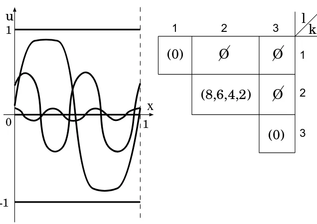
Figure 1. Wave profiles (left) and thestructureofS (right) for equation (2.4). The three horizontal lines indicate constant steady states.
We callCkl a monotone clusterifI(ukl1)> I(ukl2)>· · ·> I(uklmkl). Thecluster Ckk is called a simple cluster. We call Ckk a trivial cluster provided that
♯Ckk= 1. Note that Ckk always contains the constant steady staterk, but it
may contain other elements under certain circumstances. Next we define an order relation amongclustersin S.
Definition 2.12. Let Ck1l1, Ck2l2 be clusters. We define the order relation⊲
as follows:
Ck1l1 ⊲Ck2l2
def
⇐⇒ k1≤k2 and l1≥l2.
Let Ck1l1, Ck2l2 be clusters. If Ck1l1 ⊲Ck2l2, then we sayCk2l2 is smaller
thanCk1l1 in the order ⊲.
We define thestructureofS.
Definition 2.13. Let Ckl := ©ukl1 , ukl2, . . . , uklmkl
ª
(with mkl := ♯Ckl) be a
cluster. We call
Jkl := (I(ukl1 ), I(ukl2), . . . , I(uklmkl))
the sequence of modified Morse indices. We call
(Jkl)1≤k≤l≤N
Example 2.14. Let us investigate the structure of the waves of the following equation:
(2.4) ut=uxx+ 500(u−u3), x∈S1.
Clearly, there are three constant steady states. Letr1= 1,r2= 0 andr3=−1.
The nonlinear term depends only onu. Thus all the waves are standing waves (see Remark 2.18). A simple calculation reveals that the nonlinear term satisfies the hypothesis of Proposition D below. Thus we can see that all the clusters are
simple and monotone, using Proposition D. Since all theclusters are simple, there are precisely threeclusters: C11, C22 andC33 (wherer1∈C11,r2∈C22
and r3 ∈C33). We can see thatC11 and C33 are trivial clusters, using (i) of
Lemma F. Furthermore r1 and r3 are stable (see Remark 2.1) and I(r1) =
I(r3) = 0 (see Definition 2.7 and Remark 2.8). Thecluster C22 is monotone.
Thus Theorem C below tells us that the derivative of the nonlinear term at u=r2 gives♯C22= 4, because
3<
q d
du{500(u−u3)} ¯ ¯u
=r2
2π <4.
ThereforeC22 has three non-constant standing waves and one constant steady
state. The profile of the waves are as shown in Figure 1. We denote byu22 1 the
constant steady state inC22and byu222 ,u223 andu224 the non-constant standing
waves. We can assume that u22
1 ⊳ u222 ⊳u223 ⊳u224 , because all the clusters
are totally ordered sets. SinceC22 is monotone, we can see by (ii) and (v) of
Lemma F that I(u22
1 ) = 8, I(u222 ) = 6, I(u223 ) = 4 and I(u224 ) = 2. Therefore
thestructureofS is as shown in the table in Figure 1.
We introduce some more notation to state main theorems. Letu∈Sand let C(u) be theclustercontainingu. Define
u+:= inf{w|w > u, wis a constant steady state},
u−:= sup{w|w < u, wis a constant steady state},
and for each integer n≥0, defineun to be the smallest wave in the order ⊲
that satisfies the following: I(un) = 2n,un ⊲u, andun∈C(u). That is,
un = min⊲{v∈C(u)|v⊲u, I(v) = 2n}.
Lemma F below tells us that such un exists forn∈ {1,2, . . . ,[i(u)/2]}.
Roughly speakingu+is the constant steady state that is just aboveuin the
usual order, and u− is the constant steady state that is just below u in the
usual order.
Theorem A. Suppose that all the elements ofS are hyperbolic. Then
( i ) If the waveu is not a stable constant steady state, thenu connects to
u+,u− andun for alln∈ {1,2, . . . , I(u)/2−1}.
(ii) Furthermore ifi(u)is odd, thenudoes not connect to any other waves. Therefore the structure of S determines completely which u∈ S and
Remark 2.15. The statement (i) of Theorem A is obtained by Angenent-Fiedler [AF88] (see Proposition 6.3 of the present paper).
Theorem A’. Suppose thatf is dependent only onu, sayf =g(u), and that all the waves are hyperbolic. Letu be a wave whose Morse indexi(u) is even. Thenuconnects only tou+,u−,un (n∈ {1,2,· · ·, I(u)/2}), and everyv∈S
that satisfies the following: v ⊳u,I(v)≤I(u), and there is no wave w such
that u⊲w⊲v,I(u) =I(w), andu6=w6=v.
Remark 2.16. The structure of S tells us the modified Morse index of every wave. In the case wheref depends only onu, we can know the (real) Morse index of every wave by using Lemmas F and F’ stated below. Thus we see by Theorems A and A’ that the heteroclinic connections are determined by the
structureofS provided thatf depends only onu.
Corollary B.
♯S≥N+
N X
j=1
q
(fu(rj,0))+
2π
,
where[[y]]denotes the largest integer that is strictly smaller thany(i.e. [[y]] = −[−y]−1) and(y)+:= max{y,0}.
Remark 2.17. The hyperbolicity of the solutions is not assumed in Corollary B.
Theorem C. Suppose that all u∈S are hyperbolic. Then the following two conditions are equivalent:
(a)
(2.5) ♯S=N+
N X
j=1
q
(fu(rj,0))+
2π
,
where(y)+:= max{y,0}.
(b) all the clusters are simple and monotone.
Moreover, under these conditions, i(u) = I(u)−1 = (z(ux)−1) is odd for
any non-constant u ∈ S. Thus the hypotheses of Theorem A are satisfied. The conclusions ofTheorem Ahold. Specifically the structure ofS is uniquely determined by the sequence[[p
(fu(rj,0))+/(2π)]] (j= 1,2, . . . , N). The global
picture of heteroclinic connections in S is also uniquely determined as shown in Figure 9.
In the case wheref is dependent only onu, sayf =g(u), we introduce other two assumptions (A4) and (A5)j below. Let
(2.6) G(u) =
Z u
0
(A4) There exists an odd constant k such that G(r1) ≤ G(r3) ≤ · · · ≤ G(rk)≥G(rk+2)≥ · · · ≥G(rN),G(r2)≤G(r4)≤ · · · ≤G(rk−1) and
G(rk+1)≥G(rk+3)≥ · · · ≥G(rN−1).
If k = 1 or k = n, then the second or the third inequalities in (A4) are not assumed respectively. We will see in Section 8 that Ckl (k 6= l) is empty
provided that (A4) holds. Thus everyclusterissimple(see Figures 11 and 12). We impose the other assumption: Forj∈ {2,4,6, . . . , N−1},
(A5)j g(u)/|u|is decreasing for u∈(rj−1, rj)∪(rj, rj+1).
The condition (A5)j guarantees thatCjjismonotone(Lemma 8.1). Hence we
obtain the following:
Proposition D. Suppose that f is dependent only on u, say f =g(u), and that all the waves are hyperbolic. If (A4)holds and if(A5)j holds for all even
j ∈ {2,4,6, . . . , N −1}, then the hypotheses ofTheorem C are satisfied. Thus the conclusions of Theorems A,A’ andChold.
Remark 2.18. The equation (1.1) does not have rotating waves in the case where the nonlinear termf depends only onu. For the details, see the beginning of Section 7.
The next lemma is concerned with the structure of eachcluster.
Lemma E (Cluster lemma 1). Suppose that all u ∈ S are hyperbolic. Let
1 ≤k≤l ≤N. Let Ckl ={ukl1, ukl2, . . . , uklmkl} (mkl =♯Ckl)be a cluster and
letJkl= (I(ukl1), I(ukl2), . . . , I(uklmkl))be the corresponding sequence of modified
Morse indices. Then the following hold:
( i ) If kor l is odd and ifk6=l, thenCkl=∅.
( ii ) If k is odd, then ♯Jkk = 1. Thus Ckk is a trivial cluster. Moreover
I(ukk
1 ) = 0.
Lemma F (Cluster lemma 2). Under the same hypotheses of Lemma E, the following hold:
( i ) Every I(u) is an even integer, and I(ukl
n)−I(ukln+1) is equal to−2,0
or2 for all n∈ {1,2, . . . , mkl−1}.
( ii ) If I(ukl
n1−1) < I(u
kl
n1) = · · · = I(u
kl
n2) < I(u
kl
n2+1) (2 ≤ n1 ≤ n2 ≤
mkl−1)or if I(ukln1−1)> I(u
kl
n1) =· · ·=I(u
kl
n2)> I(u
kl
n2+1) (2≤n1≤
n2≤mkl−1), thenn2−n1 is even.
( iii ) If I(ukl
n1−1) < I(u
kl
n1) = · · · = I(u
kl
n2) > I(u
kl
n2+1) (2 ≤ n1 ≤ n2 ≤
mkl−1)or if I(ukln1−1)> I(u
kl
n1) =· · ·=I(u
kl
n2)< I(u
kl
n2+1) (2≤n1≤
n2≤mkl−1), thenn2−n1 is odd.
2
4
6
8
h(
ξ
)
η
Amplitude
[image:13.595.192.403.150.348.2]large 0
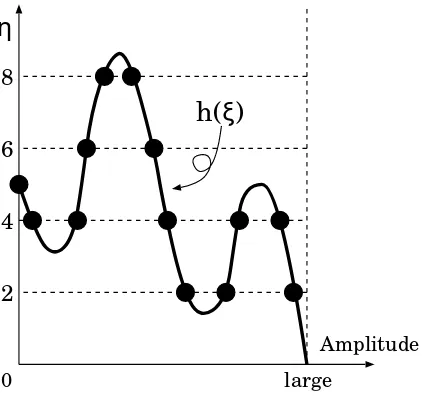
Figure 2. An example of h(ξ) mentioned in Remark 2.19. In this case, the sequence of modified Morse indices is (6,4,4,6,8,8,6,4,2,2,4,4,2).
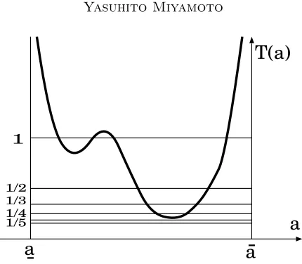
Remark 2.19. In view of Lemma F, the sequence of modified Morse indices Jkk=
¡
I(ukk j )
¢mkk
j=1 may better be illustrated as the intersection points between
the graph of a functionη =h(ξ) where 1/h(ξ) is the time-map and the hori-zontal lines η = 2,4,6,8,· · · (see Figure 2). The time-map is used in Section 3 (see the definition of T(a) in the statement of Lemma 3.1). This function h satisfies thath′(ξ)6= 0 wheneverh(ξ) is an even integer, and thath(ξ) = 0 if
ξis large.
Lemma F’ Suppose that f is dependent only on u, say f = g(u), and that all the waves are hyperbolic. Let {ukl
b1, u
kl b2, . . . , u
kl
bn} (b1 < b2 < · · · < bn)
be the non-constant waves in a cluster Ckl whose modified Morse indices are
the same number (i.e. I(ukl
b1) = I(u
kl
b2) = · · · = I(u
kl
bn)). Then i(u
kl bn−2j) = I(ukl
bn−2j)−1 (j ∈ {0,1, . . . ,[(n−1)/2]}) and i(u
kl
bn−2j−1) = I(u
kl
bn−2j−1) (j ∈
{0,1, . . . ,[(n−2)/2]}).
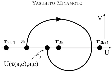
3. Proof of the Key Lemma
We will also prove three lemmas which are used in the proof of main theorems. One of these lemmas (Lemma 3.1) is the key to the present paper.
r
2k-1a
r
2kr
2k+1U(
τ
(a,c),a,c)
[image:14.595.185.406.125.265.2]U
V
Figure 3. The picture denotes the arc that starts from the point (a,0) at the time 0 and arrives at a point (b,0) (r2k−1<
b < r2k) at a certain positive time. The U-coordinate of the
arrival point is denoted by U(τ(a, c), a, c) whose meaning is specified below. The arc deforms with respect toa andc. If we select suitableaandc, then the arrival point coincides with the starting point (i.e. U(τ(a, c), a, c) =a), which means the arc is a closed orbit.
following hold:
fu(r2k,0)<0 if k∈ {1,2, . . . ,[N/2]};
fu(r2k−1,0)>0 if k∈ {1,2, . . . ,[N/2] + 1}.
Let us introduce some notation. Let u(x, t) = U(ζ) ∈ S. The wave U(ζ) should satisfy the following equation and periodic boundary conditions:
(3.1)
(
Uζζ+cUζ +f(U, Uζ) = 0, ζ∈(0,1),
U(0) =U(1), Uζ(0) =Uζ(1).
We transform the equation of (3.1) into the normal form:
(3.2)
dU dζ =V dV
dζ =−cV −f(U, V).
Let U-axis andV-axis be the horizontal and vertical axes of the phase plane respectively. First, we note that no closed orbit appears near the points (r2k−1,0) (k∈ {1,2, . . . ,[N/2] + 1}), since there points are saddle points. In
what follows we will construct closed orbits in a neighborhood of the points (r2k,0) (k∈ {1,2, . . . ,[N/2]}) on the phase plane.
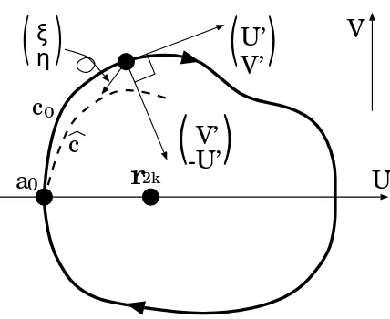
In order to explain our idea suppose that there is an orbit as shown in Figure 3. This orbit starts from the point (a,0), passes the segment (r2k, r2k+1)× {0},
and arrives at a point on the segement (r2k−1, r2k)× {0}.
band domainr2k−1< U < r2k+1. Hereafter bythe arc corresponding to (a, c)
we shall mean the portion of the orbit of (3.2) starting at (a,0) and ending at a point on the segment (r2k−1, r2k)× {0}as shown in Figure 3.
Letτ(a, c) be the arrival time of this arc; that isτ(a, c) is the smallest positive time τ such that U(τ(a, c), a, c)∈ (r2k−1, r2k) andUζ(τ(a, c), a, c) = 0 where
U(ζ, a, c) denotes the solution of (3.2) with initial data U(0) = a, V(0) = 0, and Uζ denotes the derivative of U with respect to the first variable. Clearly
the arc forms a closed orbit of (3.2) if and only if
(3.3) a=U(τ(a, c), a, c).
Furthermore this closed orbit represents a solution of (3.1) if and only if
τ(a, c) = 1 n for some n∈ {1,2, . . .}.
The following lemma shows that there is a continuous family of closed orbits corresponding to varying choice ofaandc.
Lemma 3.1. For eachr2k (k= 1,2, . . . ,[N/2]), there exists a constant a with
r2k−1≤a< r2k and a functionc=c(a)∈C1((a, r2k))such that the following
hold.
( i ) For each a∈(a, r2k), the relation(3.3)holds if and only if c=c(a).
(ii) LetT(a)be the period of the closed orbit obtained in( i ), that is,T(a) = τ(a, c(a)). Then
lim
a→aT(a) =∞, a→limr2k
T(a) = p 2π
fu(r2k,0)
.
Proof. We begin with the outline of the proof. The proof consists of three steps. In Step 1 we will show by using the bifurcation theory that there exists a family of closed orbits of (3.2) near the point (r2k,0). Thusc(a) can be defined near
a = r2k. In Step 2 we will show that whenever (a0, c0) satisfies (3.3), a C1
-functionc(a) can be defined in a neighborhood ofa0such thatc(a0) =c0. We
will use the implicit function theorem to show that. In Step 3 we will expand the domain of the functionc(a). We will define the infimumasuch thatc(a) can be defined on the interval (a, r2k). We will prove lima→r2kT(a) = 2π/
p
fu(r2k,0)
whereT(a) is the period of the closed orbit corresponding to (a, c(a)). We will also prove lima→aT(a) =∞.
Step 1: We linearize (3.2) at the point (r2k,0):
(3.4) d
dζ
µ
U V
=
µ
0 1
−fu(r2k,0) −c−fp(r2k,0) ¶ µ
U V
,
where fu and fp indicate derivatives of f with respect to the first and the
second variable respectively. Let ν± be the eigenvalues of the above matrix.
Then we have
Re(ν±) =−
c+fp(r2k,0)
2 , Im(ν±) =±
s
−fu(r2k,0) + µc+f
p(r2k,0)
2
¶2
We regardcas a parameter. Ifc=−fp(r2k,0), then the matrix is non-singular,
has the pair of simple pure imaginary eigenvalues ±iµ (µ > 0), and has no eigenvalue of the form±ikµ (k∈N, k6= 1). Moreover we can easily see that
dRe(ν±)
dc
¯ ¯ ¯ ¯c
=−fp(r2k,0) =−1
2 <0.
Therefore, (see for example Theorem 2.6 of [AP93] (Section 7, page 144)) a Hopf bifurcation occurs at c =−fp(r2k,0). Thus there are closed orbits encircling
the point (r2k,0) on the phase plane that have any small amplitude.
Step 2: From Step 1, we assume that there is a closed orbit corresponding to (a0, c0) on the phase plane. The continuity of the arc with respect toaand
c guarantees that there is a constantε >0 such that the arc corresponding to (a, c) exists as shown in Figure 3 provided that |a−a0| < εand |c−c0|< ε.
Since the solutionU(ζ) to (3.2) with initial dataU(0) =a,Uζ(0) = 0 depends
onaandccontinuously, we writeU =U(ζ, a, c). Let F(·,·) be a function as follows:
(3.5) F(a, c) :=U(τ(a, c), a, c)−a,
where τ(a, c) which is defined in the first part of Section 3 is the arrival time of the arc corresponding to (a, c). From (3.3), the arc corresponding to (a, c) is a closed orbit if and only if F(a, c) = 0. We will prove that there exists a C1-functionc(a) in a neighborhood of a
0 that satisfies F(a, c(a)) = 0. First
we see by the assumption that F(a0, c0) = 0. Second we see that U(ζ, a, c)
is a C2-function of ζ, a and c by the general theory of ordinary differential
equations. Using the equation
Uζ(τ(a+ ∆a, c), a+ ∆a, c)−Uζ(τ(a, c), a, c) = 0,
where ∆ais a small number and the definition of the derivative, we can show thatτ(a, c) is of classC1. ThusF(a, c) is of classC1. Third we will show that
Fc(a0, c0)6= 0 where
Fc(a, c) =Uζ(τ(a, c), a, c)τc(a, c) +Uc(τ(a, c), a, c).
SinceUζ(τ(a0, c0), a0, c0) = 0, we obtain
Fc(a0, c0) =Uc(τ(a0, c0), a0, c0).
We will prove in Lemma 3.2 below that
(3.6) Uc(τ(a0, c0), a0, c0)6= 0.
Now we assume that Lemma 3.2 holds. Then the implicit function theorem says that there is a C1-function c(a) that satisfies F(a, c(a)) = 0 for a ∈
(a0−ε, a˜ 0+ ˜ε) where ˜ε(>0) is so small that |c0−c(a)|< εand |a0−a|< ε
fora∈(a0−ε, a˜ 0+ ˜ε).
r
r
r
r
r
r
2k-1
2k 2k+1
2k-1
2k 2k+1
V=
V=
−δ
δ
[image:17.595.139.459.157.280.2]c>0: large
-c>0: large
Figure 4. The phase planes of (3.2) for two extreme cases. Circles in each picture are the closed orbit corresponding to (a0, c0). Ifc is large, then the arc corresponding to (a, c) (a <
a0) cannot pass the segment (r2k−1, r2k+1)× {−δ}and the
ar-rival point is in the inside of the closed orbit (the left picture). If −c is large, then the arc corresponding to (a, c) does not pass the segment (r2k, r2k+1)× {0}(the right picture).
uniquely determined. This means that there is no closed orbit corresponding to (a0, c1) (c16=c0) when there is a closed orbit corresponding to (a0, c0).
Step 3: Hereafter we suppose that there exists the closed orbit corresponding to (a0, c0). We defineaas follows:
a:= inf{a∈R|c=c(ξ) can be defined for allξ∈(a, a0)}.
Note that there is a closed orbit corresponding to (a, c(a)) for all a∈(a, a0).
We will show by contradiction that the family of closed orbit corresponding to (a, c(a)) (a∈(a, a0)) is not uniformly away from two points (r2k−1,0) and
(r2k+1,0). We assume that the family is uniformly away from two points.
We will show that there exists a constant c∗ > 0 such that the following
holds: if |c| > c∗, then a closed orbit starting from the point (a,0) (a < a 0)
does not exists.
For any δ >0, there is a constant c (>0) such that−cV −f(U, V)>0 on the segment (r2k−1, r2k+1)× {−δ}. The segment should intersect the closed
orbit corresponding to (a0, c0) provided that δ is small. If there is a closed
orbit corresponding to (a, c) (a < a0), then it should intersect the other closed
orbit and this contradicts to Lemma 4.1. Similarly, if −c (>0) is large, then there should not exist closed orbits corresponding to (a, c) (a < a0).
If the closed orbit corresponding to (a, c) (a < a0) exists, then c = c(a) is
bounded.
Let{am}∞m=1 be a sequence that satisfies the following:
Since c(a) is bounded, then there exists a constant c∗ such that the following
holds:
c(am)→c∗ as m→ ∞.
We consider the arc corresponding to (a, c∗). Let (U(ζ), Uζ(ζ)) be a closed
orbit with periodT1. ThenU(ζ) satisfies (2.1). From Lemma 3.3 below, there
is a constantM >0 such that||Uζ(ζ)|| ≤M. Thus any closed orbit is bounded
on the phase plane.
Because of the continuity of arcs with respect to aand c, the boundedness of arcs, and the assumption that the family of closed orbit is uniformly away from the two points, the arrival point of the arc corresponding to (a, c∗) exists.
Thus U(τ(a, c∗),a, c∗) can be defined. Using the continuity of U(τ(a, c), a, c)
with respect to a and c, we can obtain a contradiction if we assume that U(τ(a, c∗),a, c∗)6=a. Thus we see that
U(τ(a, c∗),a, c∗) =a.
This implies that there exists a closed orbit that contains (a,0) on the phase plane. This is a contradiction because of the definition ofaand Step 2. Thus the family is not uniformly away from the two points (r2k−1,0) and (r2k+1,0). This
means thata=r2k−1or the shortest distance of the closed orbit corresponding
to (a, c(a)) and the point (r2k+1,0) goes to zero asa→a.
We will show thatc(a) can be defined in (a, r2k). We define ¯aas follows:
¯
a:= sup{a∈R|c=c(ξ) can be defined for allξ∈(a,¯a)}.
Suppose ¯a < r2k. From Step 1 we can find ˜a with ¯a <a < r˜ 2k so that there
is a closed orbit that contains (˜a,0) on the phase plane. Since there are closed orbits with any small amplitude encircling the point (r2k,0). The functionc(a)
can be defined at some ˜a for ˜a ∈ (¯a, r2k). Using Step 2, we can expand the
domain ofc(a) to the left. Sincec(a) is unique, this contradicts to the definition of ¯a. Thus ¯a=r2k.
Since c(a) is unique and continuous, there is precisely one closed orbit that contains the point (a,0). Thus the limit lima→r2kT(a) should coincide with the limit in the statements of Theorem 2.6 in Section 7 of [AP93]. We have
lim
a→r2k
T(a) =p 2π
fu(r2k,0)
.
Hereafter we will show that lima→aT(a) =∞in the case where the
short-est distance of the family of periodic orbits and the point (r2k+1,0) goes to
zero. First, we consider the linearized eigenvalue problem of (3.2) at the point (r2k+1,0). Letλ1,λ2 be the eigenvalues. Then we have
λ1=
1 2
½
−(c+fp(r2k+1,0))−
q
(c+fp(r2k+1,0))2−4fu(r2k+1,0)
¾
,
λ2=
1 2
½
−(c+fp(r2k+1,0)) +
q
(c+fp(r2k+1,0))2−4fu(r2k+1,0)
¾
0
a
a
2 1U
[image:19.595.197.395.155.290.2]V
Figure 5. This picture indicates the phase plane displayed in the new coordinate. The thick curved arrow ( ˜U ,V˜) is the arc that we observe. Two dashed lines are directions of the two eigenvectors of the matrix. The time required for traveling through the thick part of the arc diverges asa1→0.
Because fu(r2k+1,0) <0, we have λ1 < 0 < λ2. Thus the equilibrium point
(r2k+1,0) on the phase plane is hyperbolic. Then the Grobman-Hartman
the-orem says that there is a local homeomorphism Ψ such that φt◦Ψ = Ψ◦φ˜t
and Ψ(0,0) = (r2k+1,0) where φt,φ˜t are the semiflows onR2 formed by (3.2)
and (3.4) respectively.
We can see that the time required for traveling through a neighborhood of the origin diverges as the shortest distance of the arc and the origin tends to zero. We omit the details of the proof of this fact.
We consider arcs of (3.2) in a neighborhood (r2k+1,0). For each arc
cor-responding to (a, c), there is an orbit of (3.4) that is mapped to the arc by Ψ. Since c(a) is bounded, the time which needs the orbit of (3.4) to pass a neighborhood of the origin uniformly diverges. Thus the time which needs the arc corresponding to (a, c(a)) to pass a neighborhood of the origin diverges as a→a. This means
(3.7) lim
a→aT(a) =∞.
We can prove (3.7) similarly in the case where a = r2k−1. The proof is
completed. ¤
Lemma 3.2. Let F(a, c) be the function defined by (3.5). If there is a closed orbit corresponding to(a0, c0) on the phase plane, thenFc(a0, c0)6= 0.
Proof. We use the notation used in the proof of Lemma 3.1. We assume that a closed orbit corresponding to (a0, c0) exists. Differentiating F(a, c) =
U(τ(a, c), a, c)−awith respect to cyields
a
r
U
c
c
2k
0
V
0
U’
V’
( )
-U’
V’
( )
( )
ξ
[image:20.595.190.404.155.330.2]η
Figure 6. The thick closed curve represents the closed orbit corresponding to (a0, c0) whose starting and arrival points are
(a0,0). The dashed curve represents the arc corresponding to
(a0,ˆc) (ˆc > c0) whose starting point is also (a0,0). The short
arrow represents the vector (ξ, η). This picture indicates that the vector (ξ, η) points toward the interior of the closed orbit.
We have
Fc(a0, c0) =Uc(τ(a0, c0), a0, c0),
becauseUζ(τ(a0, c0), a0, c0) = 0. We have to show thatUc(τ(a0, c0), a0, c0)6= 0.
Let ˆc (> c0) be a real number that is close to c0. Using the vector
µ
V −c0V −f(U, V)
, we can see by [Du53] that the arc corresponding to (a0, c0)
does not intersect with the arc corresponding to (a0,c) in spite that all as-ˆ
sumptions of [Du53] are not satisfied on {V = 0}. The continuity of the arc corresponding to (a, c) with respect toc, togather with the above fact, tells us that the point (U(ζ, a0,ˆc), V(ζ, a0,ˆc)) (ζ >0) is in the domain surrounded by
the closed orbit corresponding to (a0, c0). This means that U(τ(a, c), a, c) is
non-decreasing inc. We defineξandη as follows:
ξ(ζ) :=Uc(ζ, a0, c0), η(ζ) :=Vc(ζ, a0, c0),
whereUcis a derivative ofU with respect to the third variable. LetG(ζ) be the
inner product of
µ
Vζ
−Uζ 
and
µ
ξ η
. NamelyG(ζ) =ξ(ζ)Vζ(ζ)−η(ζ)Uζ(ζ).
Then we haveG(ζ)≥0, because the vector
µ
ξ η
Differentiating (3.2) with respect toc yields
(3.8)
dξ dζ =η dη
dζ =−v−cη−fu(U(ζ), V(ζ))ξ−fp(U(ζ), V(ζ))η.
Using (3.2) and (3.8), we can expressG(ζ),Gζ(ζ),Gζζ(ζ) andGζζζ(ζ) withξ,
η,c,V and derivatives off as follows: G(ζ) =−(cξV +ξf+ηV),
Gζ(ζ) =(cξV +ξf+ηV)(c+fp) +V2,
Gζζ(ζ) =(cξV +ξf+ηV)©fupV −(cV +f)fpp−(c+fp)2ª
−3cV2−V2f
p−2V f,
Gζζζ(ζ) =(cξV +ξf+ηV) £
(cV +f)2f
ppp+{4(c+fp)(cV +f)−V fu}fpp
−(4cV + 3V fp+fp)fup−V(3cV + 1)fupp
+V2fuup−V2+ (c+fp)3 ¤
−V2(V fup−cV fppf fpp)−2V(V fu−cV fp−f fp)
+ 2(cV +f)(3cV +f fpV +f).
We suppose that Uc(τ(a0, c0), a0, c0) = ξ(τ(a0, c0)) = 0. Since
V(τ(a0, c0), a0, c0) = 0, we obtain G(τ) = Gζ(τ) = Gζζ(τ) = 0 and
Gζζζ(τ) = 2f2 > 0 where τ = τ(a0, c0). Therefore, there is a small
con-stant δ > 0 such that G(P −δ) < 0. This is a contradiction, because
G(ζ)≥0. ¤
Lemma 3.3. There is a constantM >0such thatsupζ∈R|Uζ(ζ)| ≤M for any
closed orbit(U(ζ), Uζ(ζ))of (3.2).
Proof. Let (U(ζ), Uζ(ζ)) be a closed orbit of (3.2) with some c. Then U(ζ)
satisfies (2.1). Thus from (A3) there is a constant L2 > 0 such that
||U(ζ)||C1(S1)< L2 for any periodic solution or constant solution. The lemma
is proved. ¤
Lemma 3.2 completes the proof of Lemma 3.1.
4. Preparation for the Proof of Theorem A
In this section we will show that everyclusteris a totally ordered set in the order ⊲ (Corollary 4.2). We will show that z(u−v) = z(vx) provided that
u, v∈S and v⊲u(Lemma 4.4). The two lemmas are used to prove Theorem
A.
The following Lemma 4.1 is a generalized version of Corollary 4.2 below.
Lemma4.1. Let(u(x), ux(x)),(v(x), vx(x))be closed orbits on the phase plane.
We can prove Lemma 4.1 by contradiction. We omit the proof.
Using a phase plane analysis and Lemma 4.1, we immediately obtain the following corollary.
Corollary 4.2 (Matano and Nakamura [MN97]). Let u, v ∈ S. If R(u)∩ R(v)6=∅, then Int(R(v))⊃R(u) or Int(R(u))⊃R(v) where Int(R(u)) indi-cates the set consists of the interior points of R(u).
Remark 4.3. Letu, v ∈S (u6=v). By Corollary 4.2, we can see that u⊲ v
means that Int(R(u))⊃R(v).
Letu, v∈S. By using Corollary 4.2, we have eitheru⊲vorv⊲uprovided
that R(u)∩R(v)6=∅.
Corollary 4.2 and the definition of the clusters show that every cluster
is a totally ordered set. Thus we can number the elements of each cluster
©
ukl
1 , ukl2, . . . , uklmkl
ª
in such a way that ukl
1 ⊳ukl2 ⊳· · ·⊳uklmkl.
Lemma 4.4 (Matano and Nakamura [MN97]). Let u, v ∈ S. If v ⊲ u, then
z(u−v) =z(vx).
5. Proof of Corollary B and Lemmas E and F
In this section we will prove Corollary B and Lemmas E and F by using Lemma 5.1 and the results in Sections 3 and 4.
Letc=c(a) be the function defined in the statement of Lemma 3.1, and let T =T(a) be the period of the closed orbit corresponding to (a, c(a)) defined in the statement of Lemma 3.1.
Lemma5.1. Letu∈Sbe the closed orbit corresponding to(a0, c(a0))in Section
3. Ifuis hyperbolic, then∂aT(a)|a=a06= 0.
Proof. We will prove the lemma by contradiction. We assume that ∂aT(a)|a=a0 = 0. Let u(x, t) = U(ζ) (ζ = x−ct) be a rotating wave or a
steady state. We can suppose that U(0) = a and Uζ(0) = 0 without loss
of generality. The function U = U(ζ, a, c(a)) defined in Section 3 satisfies Uζζ+c(a)Uζ +f(U, Uζ) = 0. Differentiating the equation with respect to a
gives
∂ζζ(Ua+caUc) +c∂ζ(Ua+caUc) +fu·(Ua+caUc) +fp∂ζ(Ua+caUc) =−caUζ.
Letϕ(ζ) =Ua(ζ) +caUc(ζ). The functionϕ(ζ) satisfies the following equation:
(5.1) ϕζζ+cϕζ+fuϕ+fpϕζ =−caUζ, ζ∈S1.
If ca(a0) = 0, thenα·Uζ(ζ) (α∈R) are the solutions to (5.1) because of the
hyperbolicity ofU(ζ). Ifca(a0)6= 0, then (5.1) has no solution. Because 0 is a
simple eigenvalue of the following problem:
Case 1: ca(a0) = 0
Differentiating U(0, a, c(a)) =U(T(a), a, c(a)) with respect toagives (5.2) Ua(0, a, c(a)) +ca(a)Uc(0, a, c(a))
=∂aT(a)Uζ(T(a), a, c(a)) +Ua(T(a), a, c(a)) +ca(a)Uc(T(a), a, c(a)).
Substituting∂aT(a)|a=a0 = 0 andca(a0) = 0 for (5.2) givesUa(0, a0, c(a0)) =
Ua(T(a0), a0, c(a0)). SinceUa(·, a0, c(a0)) is a periodic function and the period
T(a0) is equal to 1/n for some n ∈ {1,2,· · · }, we have Ua(0, a0, c(a0)) =
Ua(1, a0, c(a0)). Sinceϕ(ζ) =Ua(ζ), we have
(5.3) ϕ(0) =ϕ(1).
We differentiate Uζ(0, a, c(a)) = Uζ(T(a), a, c(a)) with respect to a, and
substitutea0 for it. Then we obtain
Uζa(0, a0, c(a0)) =Uζa(T(a0), a0, c(a0)) +∂aT(a)|a=a0Uζζ(T(a0), a0, c(a0)).
Sinceϕζ(ζ) =Uζa(ζ, a0, c(a0)), we have
ϕζ(0) =ϕζ(T(a0)) +∂aT(a)|a=a0Uζζ(T(a0), a0, c(a0)).
Since∂aT(a)|a=a0 = 0 andϕζ(T(a0)) =ϕζ(1), we have
(5.4) ϕζ(0) =ϕζ(1).
Using (5.3) and (5.4), we can see thatϕ(ζ)(=Ua(ζ)) satisfies (5.1) and periodic
boundary conditions. By the hyperbolicity of u(x, t)(= U(ζ)), we see that ϕ(ζ) =α·Uζ(ζ) (α∈R) are the solutions to (5.1). On the other handϕ(0) =
Ua(0) = 1. It contradicts thatUζ(0) = 0. We can see that∂aT(a)|a=a0 6= 0.
Case 2: ca(a0)6= 0
Using the assumption of contradiction ∂aT(a)|a=a0 = 0, we can obtain the
following two equalities in a similar way of Case 1: (5.5) ϕ(0) =ϕ(1), ϕζ(0) =ϕζ(1).
Using (5.5), we can see thatϕ(ζ) satisfies (5.1) and periodic boundary condi-tions. The functionϕ(ζ) is a non-trivial solution to (5.1). This is a contradic-tion. Therefore, we obtain∂aT(a)|a=a0 6= 0. ¤
Hereafter, we consider the structure of each cluster. We divide theclusters
in two types. One is a type of clusters that contain a constant steady state, and the other is a type ofclustersthat do not have a constant steady state.
First, we consider the type of clusters that have a constant steady state. Since the cluster Ckl has a constant steady state, we can see that k = l by
using a phase plane analysis. If k is odd, then ♯Ckk = 1 and the element of
Ckk is a stable constant steady state. Ifkis even, then ♯Ckk ≥1 andCkk has
precisely one unstable constant steady state.
Second, we consider the type ofclustersCklthat do not have a constant steady
state. By observing the phase plane, we see thatl≥k+2, andkandlare even. If u(x, t) =U(x−ct) is an element of Ckl that satisfies (U(0), Uζ(0)) = (a,0)
1
1/2 1/3 1/4 1/5
T(a)
a
[image:24.595.189.404.126.314.2]a
a
Figure 7. The picture shows the graph ofT(a) in the case ofCkl (k6=l). Each of the intersections of the curve and the
lines corresponds to a rotating wave. In this case, the sequence of modified Morse indices is (2,2,2,4,6,8,8,6,4,2).
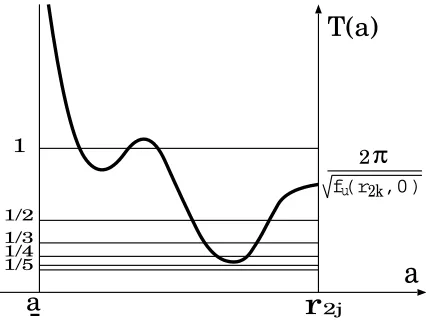
plane by using a similar way of Step 2 and Step 3 in the proof of Lemma 3.1, and enlarge the domain of c=c(a). Let (a,¯a) be the maximal connected domain of the functionc=c(a). The closed orbit that corresponds to (a, c(a)) approaches (r2k−1,0) or (r2l+1,0) asa→a. Sincec(a) is bounded, the function
T(a) diverges to +∞as a→a. The function T(a) diverges to +∞ asa→a,¯ because the closed orbit approaches (r2k,0),. . ., (r2l−1,0) or (r2l,0), andc(a)
is bounded. Hence the graph of T(a) is as shown in Figure 7.
Proof of Lemma E. The statements (i) and (ii) are easily understood by
ob-serving a phase plane. ¤
Proof of Lemma F. We can see that (i), (iv) and (v) follow from Figures 7 and
8. Lemma 3.1 implies (ii) and (iii). ¤
Proof of Corollary B. SinceS=S
1≤k≤l≤NCkl, we obtain the following:
♯S = X
1≤k≤l≤N
♯Ckl
≥
N X
j=1
♯Cjj
≥
by Figure 8N+
N X
j=1
q
(fu(rj,0))+
2π
.
1
1/2 1/3 1/4 1/5
T(a)
a
a
r
2j2
[image:25.595.191.404.150.311.2]f(r ,0)u 2k
π
Figure 8. The picture indicates the graph ofT(a) in (a, r2k).
Each of the intersections of the curve and the lines corresponds to a rotating wave. The sequence of modified Morse indices is easily computed from this picture. In this case, the sequence of modified Morse indices is (4,4,6,8,8,6,4,2,2,2).
Remark 5.2. If ♯S attains the lower bound, then every cluster is simple and
monotone. If everyclusterissimple, then the equality in the first inequality in the proof of Corollary B holds. If everyclusterismonotone, then the equality in the second inequality in the proof of Corollary B holds. Therefore,♯Sattains the lower bound if and only if everyclusterissimpleandmonotone.
6. Proof of Theorems A and C
In this section we will prove Theorems A and C by using Lemma 6.1, Lemma F and the main results of [AF88]. A simple example is given at the end of this section.
Lemma 6.1 (Blocking lemma). Let v, w∈S (w ⊲ v andI(w)< I(v)). If there exists a wave ¯v ∈ S such that w ⊲v¯ ⊲v and I(¯v) = I(w), then v does not connect to w.
The proof of Lemma 6.1 is essentially the same as the explanation after Definition 1.6 of [FR96].
Remark 6.2. Lemma 6.1 is called thezero number blocking (see Definition 1.6 of [FR96]).
We will use the following proposition to prove Theorem A.
Proposition 6.3 (Angenent and Fiedler [AF88]). Let u∈S with i(u)>0 be hyperbolic. Then
(ii) For anyn∈N,0<2n≤i(u), there exists a wave u(n) ∈S such that
u−< u(n)< u+,z(u(n)−u) = 2n, anduconnects tou(n).
We are in a position to prove Theorem A.
Proof of Theorem A. Let v be a wave in Ckl (k ≤ l) and let w be a wave
in Cmn (m ≤ n). We prove whether v connects to w or not. When there
is a connecting orbit u = u(t) that connects v and w, we can suppose that I(w)≤I(v), becausei(w) + 1≤z(u−v)≤i(v) (see Lemma 3.7 in [AF88]). If I(v) = 0, then there is no connecting orbit starting fromv. Thus we assume that I(v)>0. We can see thatkandl are odd, using a phase plane analysis.
There are two cases in general terms. In one case, w belongs to the same
clusterasv(i.e.(m, n) = (k, l)). In the other case,wbelongs to anothercluster
which does not includev(i.e.(m, n)6= (k, l)). First, we consider the case where w∈Cmn ((m, n)6= (k, l)).
Case 1: (m, n)6= (k, l)
We can divide the case into four more cases.
Case 1-1: (m, n)∈ {(k−1, k−1),(l+ 1, l+ 1)}
Since both k−1 and l+ 1 are even, the cluster Cmn has precisely one wave
(This wave is a stable constant steady state). We can see thatvconnects tow by (i) of Theorem 6.3, becausew=v+ orw=v−.
Case 1-2: (m, n)6∈ {(k−1, k−1),(l+ 1, l+ 1)} andR(Ckl)∩R(Cmn) =∅
There is a wave ¯w ∈ S (I( ¯w) = 0) between v and w in the usual order (i.e. v(x) < w(x)¯ < w(x) or w(x) < w(x)¯ < v(x)). We assume that there is a connecting orbitu(t) that connectsvandw. The functionz(u(t)−w(t)) is not¯ non-increasing in t. This is a contradiction. Therefore, the wave v does not connect to any w ∈ Cmn. Namely the wave v does not connect to any wave
of theabove clusters and below clusters in the usual order except for the two
clustersof Case 1-1.
Case 1-3: Ckl⊲Cmn
We see thati(v)∈ {I(v), I(v)−1} generally. We have i(v) =I(v)−1,
in the case that i(v) is odd. We suppose that there is a connecting orbitu(t) that connectsv andw. Then
(6.1) z(u−v)≤i(v),
(see Lemma 3.7 in [AF88]). Lemma 4.4 tells us that (6.1) contradicts that z(u(t)−v(t)) = I(v) for large t > 0. The wave v does not connect to any w ∈ Cmn. Namely v does not connect to any wave of the clusters that is
smaller than Ckl in the order⊲.
Case 1-4: Cmn⊲Ckl
There is a ¯w ∈ S (I( ¯w) = 0) such that R(v)∩R( ¯w) = ∅ and w ⊲ w. We¯
The Case 1 can be summarized as follows: If v connects to w in another
cluster, thenwshould bev+ or v−.
Case 2: (m, n) = (k, l)
Letwbe another wave of the sameclusterCkl. We divide this case in two more
cases.
Case 2-1: v⊲w
We suppose that there is a connecting orbit u(t) that connects v and w. We can see that
I(v) =z(u(t)−v(t))≤i(v) for larget,
(see Lemma 3.7 in [AF88]), because v ⊲ w. Thus if i(v) is odd (i.e. i(v) =
I(v)−1), then we obtain a contradiction. The waveudoes not connect tow provided thati(v) is odd.
Case 2-2: w⊲v
Owing to Theorem 6.3, the wave v connects to w that attains the following minimum for each d(d= 2,4,6, . . . , I(v)−2):
min
I(w)=2d,w⊲v|R(w)|,
where |R(u)| := maxx∈S1u(x, t)−minx∈S1u(x, t). Suppose i(v) is odd. The
wavev, however, does not connect to any otherw, because Lemma F tells us that there exists a wave ¯wsuch that w⊲w¯ ⊲v and I(w) = I( ¯w). Thus we
can see by Lemma 6.1 that the zero number blocking occurs.
The Case 2 can be summarized as follows. The wavevconnects toI(v)/2−1 different waves that are bigger thanvin the order ⊲in the samecluster. The
wave does not connect to any other wave in the sameclusterprovided thati(v) is odd.
The Case 1 and the Case 2 cover all the combinations ofv andw. Thus the
proof is completed. ¤
Proof of Theorem C. We show that the hypotheses of Theorem C satisfy those of Theorem A.
Everyclusterissimpleandmonotoneif and only if♯Sattains the lower bound (see Remark 5.2).
We will show that the Morse index of every wave is odd or zero. Suppose that there is a wave u ∈ S whose Morse index is even and not zero. Using Proposition 6.3, we can see that there exists a wavev∈Ssuch thatI(u) =I(v) and uconnects to v heteroclinically. However, u and v are not in the same
cluster, because the cluster is monotone. Thus v belongs to another cluster. However, there is no heteroclinic connection, because everyclusterissimpleand there should be a stable steady state betweenuandvin the usual order. This is a contradiction. Therefore all the hypotheses of Theorem A are satisfied. ¤
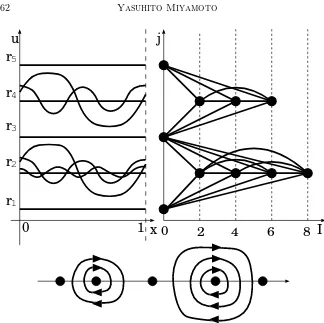
Example 6.4. Figure 9 shows the profile of every u ∈ S and the diagram that shows which u ∈ S and v ∈ S are connected heteroclinically and which are not when {rj}5j=1 are the roots of f(·,0), [[
p
fu(r2,0)/(2π)]] = 2,
[[p
I
j
2
4
6
8
r
54
3
2
1
r
r
r
r
u
x
[image:28.595.131.455.123.446.2]0
1
0
Figure 9. In the left figure, the thick curves and the lines indicate the profile of all the waves that move to the right or the left at each constant speed. In the right figure, the horizontal axis indicates the modified Morse index and the vertical axis indicates the suffix of Cjj. The points mean elements of S.
The thick curves and the lines represent the connecting orbits. The lower figure shows closed orbits and equibrium points in theuux-plane. Note that they do not necessarily correspond
to the same value ofc.
Remark 6.5. If there is a wave v ∈ S such that i(v)(6= 0) is even, then we cannot determine by the method used in the proof of Theorem A whether v connects to waves that are smaller thanv in the order⊲or not.
7. Proof of Theorem A’ and Lemma F’
In this section we will study the case where the nonlinear termfdepends only onu, and establish a sufficient condition that guarantees that all theclusters
aresimpleandmonotone.
We will use a charactergto denote the nonlinear term (i.e. f(u, ux) =g(u)).
In this case (1.1) is written as follows:
(7.1)
(
ut=uxx+g(u), x∈S1,
u(x,0) =u0(x), x∈S1.
Matano [Ma88] showed that (1.1) does not have rotating waves provided that f(u, p) =f(u,−p). Since the nonlinear term gdepends only onuand satisfies this property, the equation (7.1) does not have rotating waves.
We consider the following Neumann problem:
(7.2)
(
ut=uxx+g(u), x∈(0,1/2),
ux(0) = 0 =ux(1/2).
Letu(x) be a wave of (7.1). Then there exists θ(∈S1) such thatu
x(θ) = 0
and u(x) ≤ u(θ) for all x ∈ S1. We can see by a phase plane analysis that
ux(θ+ 1/2) = 0. Therefore u(x+θ) (0< x <1/2) is a steady state of (7.2).
Let ˜u(x) denotesu(x+θ). Thus ˜u(x) is a steady state of (7.2).
Next, let v(x) be a non-constant steady state of (7.2) that satisfiesv(x)≤ v(0). Thenu(x) is a standing wave of (7.1) where
u(x) =
(
v(x), 0≤x≤1/2; v(1−x), 1/2≤x≤1.
We can identify any waveuof (7.1) with a steady state ˜uof (7.2), and bythe steady state associated with uof (7.2) we shall mean ˜u. In short ˜u=v.
Letv, w be steady states of (7.1) and let ˜v, ˜w be steady states associated with v, w respectively. Suppose that a heteroclinic orbit ˜u(x, t) of (7.2) that connects ˜v and ˜wexists. Thenu(x, t) is a solution of (7.1) where
u(x, t) =
(
˜
u(x, t), 0≤x≤1/2; ˜
u(1−x, t), 1/2≤x≤1.
Moreoveru(·, t)→v(x) (t→ −∞) andu(·, t)→w(x) (t→ ∞). Thusu(x, t) is a connecting orbit of (7.1) that connectsvandw. In short,v connects tow if ˜v connects to ˜w. We will use this fact to prove the existence of connecting orbits in the proof of Theorem A’.
We give two lemmas about (7.2) without proofs.
Lemma7.1. Let {ukl
1, ukl2, . . . , uklmkl} be a cluster and let{u˜
kl
1,u˜kl2, . . . ,u˜klmkl}be
the set of steady states of (7.2) associated with the waves of the cluster. Let
{ukl b1, u
kl b2, . . . , u
kl
bn} (b1< b2 <· · · < bn)be the waves whose Morse indices are
the same number (i.e. I(ukl
b1) = I(u
kl
b2) = · · · = I(u
kl
bn)). Then i(˜u
I(ukl
bn−2j)/2 forj∈ {0,1, . . . ,[(n−1)/2]}, andi(˜u
kl
bn−2j−1) =I(u
kl
bn−2j−1)/2 + 1
forj∈ {0,1, . . . ,[(n−2)/2]}.
Proof. In the case of the Dirichlet problem, we can find the proof in Lemma 2.1 of [BF89]. We can prove the lemma in a similar way. ¤
Lemma 7.2. Let u,v, wbe waves and let u˜,v˜ be the steady states associated with u, v. If i(u) is even, then the steady state u˜ connects to every v˜ that satisfies the following: u⊲v, and there is no wavew such thatu⊲w⊲v and
I(u) =I(w).
Proof. In the case of the Neumann problem, the problem of the heteroclinic connections are completely determined by [FR96]. We can prove the lemma by using Lemma 7.1, Definition 1.6 of [FR96] and Lemma 1.7 of [FR96]. ¤
Proof of Lemma F’. If bn−2j > 1, then there exists v (⊳uklbn−2j) such that v blocks the connections fromukl
bn−2j to all the wave that are smaller thanu
kl bn−2j in the order⊲. This means thati(uklb
n−2j) =I(u
kl
bn−2j)−1. Ifbn−2j= 1, then k=l. There also exists a wave vthat satisfies the above conditions (the wave v may be a constant steady state). Thusi(ukl
bn−2j) =I(u
kl
bn−2j)−1. In short i(ukl
bn−2j) =I(u
kl
bn−2j)−1 for j∈ {0,1, . . . ,[(n−1)/2]}. We consider whether i(ukl
bn−2j−1) = I(u
kl
bn−2j−1) − 1 or i(u
kl
bn−2j−1) =
I(ukl
bn−2j−1). If n−2j −1 > 1, then ˜u
kl
bn−2j−1 connects to ˜u
kl
bn−2j−2. Thus
ukl
bn−2j−1 connects to u
kl
bn−2j−2. This means that i(u
kl
bn−2j−2) =I(u
kl
bn−2j−1). If
n−2j−1 = 1, then there exists a wave ˜vsuch that the following hold: v⊳uklb
1
and ˜ukl
b1 connects to ˜v. Thusu
kl
b1 connects tov. Hencei(u
kl b1) =I(u
kl
b1). In short
i(ukl
bn−2j−1) =I(u
kl
bn−2j−1) forj∈ {0,1, . . . ,[(n−2)/2]}.
¤
Proof of Theorem A’. Letube a non-constant wave whose Morse index is even. In Theorem A we have identified waves that are connected byuand that satisfy z(u−v)≤I(u)−2. Thus we have to check whetheruconnects tovor not, in the case wherez(u−v) =I(u).
Case 1: v⊲u
Letwbe a wave that satisfies the following: wis the smallest wave in the order
⊲that satisfiesw⊲uandI(u) =I(w). Because of Lemma F’, wexists in the
clusterto whichubelongs, andi(w) =I(w)−1. Let ˜uand ˜wbe steady states of (7.2) associated with uand wrespectively. We can see that ˜uconnects to
˜
w (see Case 2-1 in the proof of Lemma F’). Thus uconnects tow. There is no other wave that is connected byu, becausewblocks other connections (see Lemma 6.1).
Case 2: v⊳u
Since v ⊳ u, it is automatically satisfied that z(u−v) = I(u). If there is a
wavew such thatu⊲w⊲v and I(u) =I(w), then udoes not connect to v
2
4
6
8
Amplitude
large 0
B A
C
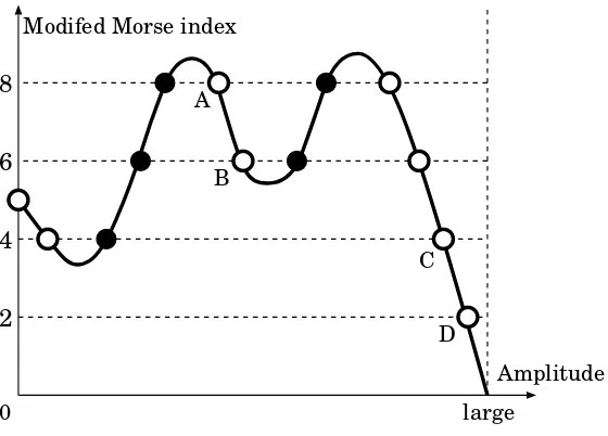
[image:31.595.158.438.150.351.2]D Modifed Morse index
Figure 10. Each black point indicates a wave whose Morse index is even (i.e. i(ukl
j ) =I(uklj )) and each white point
indi-cates a wave whose Morse index is odd (i.e. i(ukl
j ) =I(uklj )−1).
The point A connects only to B, C, D and two constant steady states.
is no such wave, thenuconnects tovbecause ˜uconnects to ˜v(see Lemma 7.2).
Therefore the theorem is proved. ¤
Example 7.3. LetJkl =¡I(uklj ) ¢mkl
j=1 (k6=l) be a sequence of modified Morse
indices. Figure 10 represents the sequence of modified Morse indices Jkl (see
Remark 2.19). Since k 6=l, we see by (v) of Lemma F that I(ukl
mkl) = 2. If i(u) is odd, all connections toward a smaller wave in the order⊲(i.e. toward
the left in Figure 10) are blocked. Ifi(u) is even, the connections to a smaller wave in the order⊲are not necessarily blocked.
8. Proof of Proposition D
In this section we consider the case where the nonlinear term does not depend onux(see (7.1)). We will use the notation used in Section 7.
We will show a sufficient condition that guaranteesclustersto be monotone. The following lemma is well-known:
Lemma8.1. Supposeg(·)has exactly three roots{ri}3i=1andr1< r2= 0< r3.
If g(u)/|u| is decreasing for u ∈ (r1,0)∪(0, r3), then there are only three
monotone clusters.
k=1
1<k<n
k=n
Figure 11. The graph of G(r); k = 1 (left), 1 < k < n (center) andk=n(right).
We will prove Proposition D after we state some definitions and notation. Hereafter, we assume that every wave of S is hyperbolic. Henceg′(r
j)6= 0 for
allj∈ {1,2, . . . , N}. The pointG(rj) (j∈ {1,3,5, . . . , N}) is a local maximum
point andG(rj) (j∈ {2,4,6, . . . , N−1}) is a local minimum point whereG(r)
is defined by (2.6).
First, we define a set of intervals
W(r) :={ρ|G(ρ)< r}. We impose the following condition of the functionG:
(A6) Let I be a bounded connected component of W(r) for r ∈ R. Let
J ={rk, rk+1, . . . , rl−1, rl} (1≤k≤l≤N). IfI⊃J, then♯J = 1.
The closed curves described as{(u, v)|v2+ 2G(u) = constant} on the phase
plane are candidates of steady state solutions of (7.1). If (A6) holds, then Ckl (k6=l) is empty. Therefore, when (A6) holds, there is only one possibility
which is the condition (A4) in Section 2. When (A4) is satisfied, the graph of G(r) looks like one of Figure 11.
Example 8.2. If the graph ofG(r) is as shown in the center of Figure 11, the corresponding phase portrait is as shown in Figure 12.
If (A4) holds, then every cluster issimple. If (A5)j holds, thenCjjis
mono-tone. Now we can prove Proposition D.
Proof of Proposition D. If (A4) holds, then (A6) holds. Thus everyCkl(k6=l)
is empty. Namely all the clusters are simple. After all S =SNj=1Cjj. Since
every wave is hyperbolic, theclusterCjj(j ∈ {1,3,5, . . . , N}) has precisely one
Figure 12. The picture indicates the phase portrait when G(p) is as shown in the center of Figure 11. The thick closed curves indicate the closed orbits which correspond to stand-ing waves, and the points indicate equilibrium points which correspond to constant steady states.
every cluster is monotone. Therefore, all the hypotheses of Theorem C are
satisfied. The proof is completed. ¤
After completing this work, the author has been informed about the pa-per [FRW04] written by Fiedler, Rocha and Wolfrum. They have given the necessary and sufficient conditions whether any pair of waves is connected het-eroclini