Fuˇc´ık spectra for vector equations
C. Fabry
Universit´e Catholique de Louvain, Institut de Math´ematique Pure et Appliqu´ee,
Chemin du Cyclotron, 2 , B-1348 Louvain-la-Neuve, Belgium e-mail:[email protected]
Abstract. — Let L : domL ⊂L2(Ω;RN) → L2(Ω;RN) be a linear
opera-tor, Ω being open and bounded in RM. The aim of this paper is to study the
Fuˇc´ık spectrum for vector problems of the form Lu=αAu+−βAu−,where A
is anN×N matrix, α, βare real numbers,u+a vector defined componentwise
by(u+)
i = max{ui,0}, u− being defined similarly. With λ∗ an eigenvalue for
the problem Lu = λAu , we describe (locally) curves in the Fuˇc´ık spectrum passing through the point (λ∗, λ∗), distinguishing different cases illustrated by
examples, for which Fuˇc´ık curves have been computed numerically.
Key words:Nonlinear eigenvalue problems, asymmetric nonlinearities.
AMS Classification:34B15, 35P30.
1
Introduction
Since the pioneering work of Dancer [5] and Fuˇc´ık [7, 8], problems with asymmetric nonlinearities, also called jumping nonlinearities, have been the subject of numerous studies. Most of these problems have the form
Lu=αu+−βu−+g(·, u), (1)
where L is a differential operator acting on a space of real-valued functions, u+ = max{u,0}, u− = max{−u,0}, and g is a supplementary nonlinear
The first question with respect to such problems is to determine the set of pairs (α, β)∈R2 for which the homogeneous equation
Lu=αu+−βu− (2)
has nontrivial solutions. These points form the so-called Fuˇc´ık or Dancer-Fuˇc´ık spectrum.
The degree of difficulty of the full problem (1) depends on whether (α, β) belongs or not to the Fuˇc´ık spectrum. If not, the existence of solutions for (1) can be easily studied through the computation of a degree for the nonlinear operator associated to equation (2) (see [1] for some recent results concerning degree computations). The more difficult case, when (α, β) belongs to the Fuˇc´ık spectrum, can be considered as a situation of resonance. Such problems have been studied, for instance, by Gallou¨et and Kavian [9], Schechter [16], Ben-Naoum, Fabry and Smets [2].
The aim of the present paper is to study Fuˇc´ık spectrum for vector equa-tions, the formulation being as follows. Let L : domL ⊂ L2(Ω;RN) →
L2(Ω;RN) be a linear operator, Ω being open and bounded in RM and A a
real N ×N matrix. We consider the equation
Lu=αAu+−βAu− (3)
(we use the same notation for the matrix and the bounded operator on L2(Ω;RN) associated to it). The notations u+, u− have to be understood
componentwise, i.e. (u+)
i = max{ui,0}, (u−)i = max{−ui,0}. The points
(α, β) ∈R2 for which (3) has nontrivial solutions form the Fuˇc´ık spectrum,
which will be denoted by Σ(L, A). With η = (α +β)/2, ǫ = (α − β)/2, equation (3) can be rewritten as
Lu=ηAu+ǫA|u|, (4)
where the absolute value|u|is again to be understood componentwise. Notice that, although we will consider below problem (3) or, equivalently (4), the discussion could easily be generalized by replacing (4) by
Lu=ηAu+ǫB|u|,
B being another real N ×N matrix.
devoted to a reduction of (3) to a finite-dimensional problem, which is valid for points (α, β) “not too far” from the diagonal in the (α, β)-plane. Using implicit function theorems, we present in Sections 3 and 4, local existence results for Fuˇc´ık curves (i.e. curves which are contained in the Fuˇc´ık spec-trum) near the diagonal α = β, distinguishing the case of curves which are transversal with respect to the diagonal, and the case of curves tangent to the diagonal; both cases are illustrated by examples. In Section 5, we consider hypotheses on L and A, under which a variational formulation can be given for the problem, the points of the Fuˇc´ık spectrum being then associated to critical values of some functional, whereas in Section 6, we introduce a condi-tion under which the Fuˇc´ık spectrum, near an interseccondi-tion with the diagonal α =β, reduces locally to a single curve perpendicular to the diagonal at the point of intersection.
The information obtained concerning the slopes of the Fuˇc´ık curves at their crossing point with the diagonal, is used as a starting point for numer-ical computations that have been performed to draw Fuˇc´ık curves for the examples considered in the paper.
2
Reduction to an equivalent problem
The points of the form (α, α) clearly play a major role within the Fuˇc´ık spectrum. They correspond to (generalized) eigenvalues λ for the equation
Lu=λAu . (5)
Let λ∗ be a particular solution of the eigenvalue problem (5). The following
hypotheses are assumed to hold throughout:
(H1) λ∗ is an eigenvalue for the pair (L, A) ; L−λ∗A is a
Fred-holm operator of index 0,which means that Im(L−λ∗A) is closed,
ker(L−λ∗A) and (Im(L−λ∗A))⊥ having the same finite
dimen-sion.
Let the adjoint of L be denoted by L∗ and the transpose of A by At; the
orthogonal projectionsP, Qonto ker(L−λ∗A) and ker(L∗−λ∗At) = (Im(L−
λ∗A))⊥ respectively, will play an important role in the sequel. The scalar
product inRN will be denoted by (·,·),whereash·,·iandk · kwill denote the
Using a Lyapunov-Schmidt decomposition, we will reduce equation (3) to a problem in a finite-dimensional space. Similar results can be found in [1] and [14] for scalar equations. Since the operator
˜
Lλ∗A= (L−λ∗A)|(ker(L−λ∗A))⊥ : (ker(L−λ∗A))⊥→Im(L−λ∗A)
admits a bounded inverse, we can prove the following lemma, wherek( ˜Lλ∗A)−1k
and kAk denote operator norms.
Lemma 1. Assume that (H1) holds and that α, β ∈R satisfy the condition
(|β−λ∗|+|α−λ∗|)k( ˜Lλ∗A)−1kkAk<1. (6)
Then, for any x∈ker(L−λ∗A), the problem
Lu = λ∗Au+ (I−Q)[αAu+−βAu−−λ∗Au], (7)
P u = x (8)
has a unique solutionux =ux(α, β). Moreover, the solutionux(α, β)is locally
Lipschitzian with respect to x, α, β.
Proof. We see that the system (7), (8) is equivalent to
u=x+ ( ˜Lλ∗A)−1(I−Q)[αAu+−βAu−−λ∗Au]
or
u=x+ ( ˜Lλ∗A)−1(I−Q)[(α−λ∗)Au+−(β−λ∗)Au−].
Condition (6) implies that, given x∈ker(L−λ∗A), the mapping appearing
on the right-hand side of the above equation is a contraction mapping. The conclusion then follows from classical results concerning contraction map-pings.
Letux =ux(α, β) be the solution of (7), (8). Define :
c0(x, α, β) = −Q[αAu+x −βAu−x −λ∗Aux]
=−α−β
2 QA|ux| −
α+β
2 −λ
∗
!
QAux,
so that ux verifies
For given α, β, equation (3) admits a nontrivial solution if and only if there exists x ∈ ker(L−λ∗A), x 6= 0, such that c
0(x, α, β) = 0. The problem is
therefore reduced to a problem in a finite-dimensional space. Notice that
ux=x+O(|β−λ∗|+|α−λ∗|) for (α, β)→(λ∗, λ∗),
uniformly for x in a bounded set, and that c0(rx, α, β) =rc0(x, α, β) for all
r ≥0.
Determining the Fuˇc´ık spectrum in the neighborhood of (λ∗, λ∗) thus
consists in finding values of (α, β),close to (λ∗, λ∗), such thatc
0(x, α, β) = 0
for some x6= 0. Using implicit function theorems, we treat that question in Sections 3 and 4, distinguishing two different cases.
3
Fuˇ
c´ık curves transversal to the diagonal
α
=
β.
In order to determine curves in the neighborhood of (λ∗, λ∗), which belong
to the Fuˇc´ık spectrum Σ(L, A), we consider the system
Lu=αAu+−βAu−,kuk= 1. (10)
As we are interested in values of (α, β) in the Fuˇc´ık spectrum, close to (λ∗, λ∗),
we let ε = (α−β)/2,(α+β)/2 =λ∗+εη; ε will be a small parameter. The
system (10) can be written
Lu=λ∗Au+εA|u|+εηAu,kuk= 1 ;
we aim at determining, for ε “small”, u, η as functions of ε satisfying the above equations. For ε6= 0, it is equivalent to
u = P u+ε( ˜Lλ∗A)−1(I−Q)[A|u|+ηAu] +JQ[A|u|+ηAu], (11)
kuk= 1,
whereJ is an isomorphism between (Im(L−λ∗A))⊥and ker(L−λ∗A).Using
the reduction of Section 2, it is also equivalent, for ε 6= 0, to the finite-dimensional problem
(in which ux depends of course on ε, η). Working as in [1], we will apply an
implicit function theorem to the problem (11), in order to solve it foru, η as functions ofε, forεclose to 0 (a similar approach has been used by Pope [14]; implicit function theorems also appear in [4] for studying the Fuˇc´ık spectrum of fourth order differential operators). For ε = 0, the equation (11) or (12) reduces to
QA|x|+ηQAx= 0, x∈ker(L−λ∗A),kxk= 1. (13)
Notice that, if (x0, η0)∈ker(L−λ∗A)×R denotes a solution of (13), and if
QAx0 6= 0, the valueη0 can be computed from
η0 =−h
A|x0|, QAx0i
kQAx0k2
. (14)
In the application of an implicit function theorem, a difficulty lies in the fact that the set of points, at which the mapping u 7→ QA|u| is differentiable, need not be open in L2(Ω;RN). That difficulty can be overcome by using a
version of the implicit function theorem that only requires a (strong) Fr´echet differentiability at one point (see [1]). The only term that needs to be con-sidered in (11) is the term JQA|u|. The required differentiability property will be based on the fact, proved by adapting an argument of [17], that, with
˜
Q a projection onto a finite dimensional space X ⊂ L2(Ω;R), the mapping
L2(Ω;R) → X : U 7→ Q˜|U|, is strongly Fr´echet-differentiable at the point
U0, provided that the real-valued function U0 does not vanish on a set of
non-zero measure. Since components of u that never contribute to QAucan be ignored, we introduce the following hypothesis:
(H2) for each i = 1,· · ·, N, the ith-component of x0 does not
vanish on a set of positive measure, unless, for anyu∈L2(Ω;RN),
the ith-component of u brings no contribution toQAu.
With (H2), the mappingu7→QA|u|is strongly differentiable atx=x0,as a
mapping from L2(Ω;RN) to (Im(L−λ∗A))⊥.The application of the implicit
function theorem yields the following result, in which (15) represents the invertibility of the Fr´echet derivative and implies QAx0 6= 0 ; sgn(x0)y is a
vector whoseith component isy
i,multiplied by the (not necessarily constant)
sign of the ith component ofx
0.If a component (x0)i of x0 vanishes on a set
of positive measure, sgn((x0)i) is undefined, but this does not matter since,
Theorem 1. Let L : domL ⊂ L2(Ω;RN) → L2(Ω;RN), A and λ∗ satisfy
hypotheses (H1),(H2). Let (x0, η0) be a solution of (13), such that
y ∈ker(L−λ∗A),hy, x
0i= 0,
Q(Asgn(x0)y) +η0QAy+µQAx0 = 0
)
=⇒y= 0, µ = 0. (15)
Then, there exist functions η(·), u(·) defined in a neighborhood E of 0, such that
u(0) =x0, η(0) =η0 =−h
A|x0|, QAx0i
kQAx0k2
, (16)
Lu(ε) = (λ∗+εη(ε))Au(ε) +εA|u(ε)|,ku(ε)k= 1, for ε∈ E. (17) Moreover, if
QAx6= 0,∀x∈ ker(L−λ∗A), x6= 0, (18) and if (15) holds for all (η0, x0) satisfying (13), the Fuˇc´ık spectrum, within a
neighborhood U of (λ∗, λ∗), consists of a finite number of curves of the form
(λ∗+ε(η(ε) + 1), λ∗+ε(η(ε)−1)),where η(0) is such that (13) has a solution
x0 for η=η(0).
Proof. As indicated above, the existence of functionsη(·), u(·) verifying (16), (17) follows from the application of an implicit function theorem to the sys-tem (12). For details, we refer to an analogous proof in [1].
For the last part of the theorem, let (αn, βn) belong to the Fuˇc´ık spectrum,
with αn→λ∗, βn →λ∗ forn → ∞.Letεn= (αn−βn)/2.Because of (18), it
is easily shown that λ∗ is an isolated eigenvalue of (L, A); hence, forn large,
we must have εn 6= 0. Let then ηn be defined by (αn+βn)/2 = λ∗ +εnηn.
The point (αn, βn) being in the Fuˇc´ık spectrum, we must have
Q(A|uxn|) +ηnQ(Auxn) = 0,
for some xn in ker(L−λ∗A),kxnk = 1. Passing to a subsequence, we can
assume that {xn} converges to some x∗ ∈ ker(L−λ∗A),kx∗k = 1. It then
follows that {ηn} must converge to
η∗ =−hA|x
∗|, QAx∗i
kQAx∗k2
and that (η∗, x∗) must be a solution of (13). Because of (15), the solutions
When condition (15) is fulfilled, the above theorem asserts the existence
the number of solutions of (13). Moreover, it is clear that, if the conditions of Theorem 1 are satisfied, the same is true with η0, x0 replaced by−η0,−x0.
Consequently, the Fuˇc´ık curves can be grouped by pairs of curves of reciprocal slopes at (λ∗, λ∗),if their slopes are different from−1.Examples with multiple
curves have been given in [1] for self-adjoint problems for scalar differential equations.
On the other hand, under (18), it follows from the last part of the proof ((15) is not required here) that, given δ > 0, there is a neighborhood of (λ∗, λ∗), such that, within that set, no point of the Fuˇc´ık spectrum, except and the equation (13) then gives two possibilities for η0 :
η0 =±h
A|x∗|, y∗i
hAx∗, y∗i .
We thus have, in the neighborhood of (λ∗, λ∗), two curves (not necessarily
distinct) in the Fuˇc´ık spectrum Σ(L, A), whose slopes are given by
±hA|x∗|, y∗i − hAx∗, y∗i
±hA|x∗|, y∗i+hAx∗, y∗i. (20)
Fuˇc´ık spectra for scalar self-adjoint problems have been the most widely studied, starting from the classical periodic and Dirichlet boundary value problems for 2nd-order ordinary differential equations [5, 7, 8]. Examples of
4th-order problems are considered in [4, 12]. The following example, taken
Example 1. Consider the scalar boundary value problem
u′′′+αu+−βu−= 0, (21)
u(0) =u′(0) =u(1) = 0. (22)
Let the operatorL be defined by
L: domL⊂L2((0,1);R)→L2((0,1);R) :u7→ −u′′′,
where domL is the set of functions in H3((0,1);R) verifying the boundary
conditions; the matrix A is simply the number 1 here. The eigenvalues of L are simple, the ith eigenvalue λ
i being equal to −τi3, where τi is the ith zero
of the function
z(s) = 1 3
"
e−s+ 2es/2sin
√
3 2 s−
π 6
!#
;
the corresponding eigenfunction is ui(t) = z(λ1i/3t). There are two Fuˇc´ık
curves emanating from each eigenvalue; they have been computed numeri-cally in [10]. According to (20), the slopes of the Fuˇc´ık curves starting from (λi, λi) are given by
±h|ui|, wii − hui, wii
±h|ui|, wii+hui, wii
, (23)
where wi is an eigenfunction of the adjoint problem
−u′′′−λiu= 0,
u(0) =u(1) =u′(1) = 0.
For the first eigenvalue, the problem (21), (22) has solutions of constant sign; hence, the Fuˇc´ık spectrum contains the lines α =λ1, β =λ1.For the second
eigenvalue, the numerical values obtained from (23) for the slopes at (λ2, λ2)
are −0.98411 and−1.01615 (the two curves are very close together, as shown in [10]); for the third eigenvalue, the values are −0.46108 and −2.16882.
4
Fuˇ
c´ık curves tangent to the diagonal
α
=
β.
(H3) dim[QA(ker(L−λ∗A))] = dim(Im(L−λ∗A))⊥−1.
Taking into account the fact that dim ker(L−λ∗A) = dim(Im(L−λ∗A))⊥,
under (H3),there exists x∗ ∈ker(L−λ∗A),kx∗k= 1, y∗ ∈ (Im(L−λ∗A))⊥,
ky∗k= 1, such that
QAx∗ = 0 andhAx, y∗i= 0,∀x∈ker(L−λ∗A).
The definition of new variables will be slightly different from Section 3; we will let now ε= (α+β)/2−λ∗, εη= (α−β)/2, and again try to determine
u, η as functions of ε, forε “small”. By analogy with (12), the equations to solve can be written, for ε 6= 0, as
ηQA|ux|+QAux = 0,kuxk= 1. (24)
For ε= 0, that system reduces to
ηQA|x|+QAx= 0, x∈ker(L−λ∗A),kxk= 1 ;
it admits the solutions (x∗,0) and (−x∗,0). Under the assumption
(H4) hA|x∗|, y∗i 6= 0,
we can apply an implicit function theorem and conclude that (24) can be solved in η, xfor ε “small”, leading to the following result.
Theorem 2. Let L : domL ⊂ L2(Ω;RN) → L2(Ω;RN) and λ∗ satisfy
hy-pothesis (H1),(H3) and (H4). Then, there exist functions η(·), u(·), v(·),
de-fined in a neighborhood E of 0, such that
(i) u(0) =x∗, v(0) =−x∗, η(0) = 0,
(ii) Lu(ε) = (λ∗+ε)Au(ε) +εη(ε)A|u(ε)|,
Lv(ε) = (λ∗+ε)Av(ε) +εη(ε)A|v(ε)|, for ε∈ E.
Under the hypotheses of Theorem 2, there are locally (at least) two Fuˇc´ık curves emanating from (λ∗, λ∗) and tangent to the line α=β,sinceη(0) = 0.
However, it is clear that no Fuˇc´ık curve transversal to the diagonal can exist when
QAx= 0, QA|x| 6= 0, for all ∈ker(L−λ∗A), x6= 0,
whereas, as already pointed above, there is no Fuˇc´ık curve tangent to the diagonal when
For the operatorL, we take
L: domL⊂L2((0,1);R2)→L2((0,1);R2) : u
domL being the set of functions in H1((0,1);R2) verifying the boundary
conditions. With
integer; they are simple, the corresponding eigenfunctions being given by
wn(t) = cos(2n+ 1)t
−sin(2n+ 1)t
!
.
The same wn are also eigenfunctions for the adjoint problem. It is easy to
check that hAwn, wni= 0, whereas
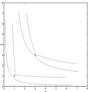
Hence, Theorem 2 applies and, consequently, two Fuˇc´ık curves tangent to the diagonal α = β pass through the points (λn, λn). Two pairs of such curves
0 1 2 3 4 5 6 7 8 0
1 2 3 4 5 6 7 8
α
β
Figure 1: Fuˇc´ık curves for the problem (25), (26).
5
Problems with a variational structure
We will now discuss situations where the problem has a variational structure and will study the Fuˇc´ık spectrum in a squareI×I,whereIis a closed interval such that the contraction condition (6) of Lemma 1 is satisfied for any α, β in I. We will assume that the operator L is self-adjoint, and the matrix A diagonal. These hypotheses may seem very restrictive, but the required structure may of course be obtained after a multiplication of equation (3) by an invertible matrix T chosen to makeT Lself-adjoint andT Adiagonal. We define the functional
h0 : ker(L−λ∗A)×I×I →R : (x, α, β)7→ hc0(x, α, β), xi.
Notice that, L−λ∗A being self-adjoint, the projectors P = Q coincide, so
that, using (9), we have
h0(x, α, β) = hc0(x, α, β), xi=hc0(x, α, β), uxi,
= hLux, uxi −αhAu+x, uxi+βhAu−x, uxi.
or, since A is assumed diagonal,
The next lemma presents a few properties of the functions c0 and h0.
Lemma 2. Assume that the operator L : domL ⊂ L2(Ω;RN) → L2(Ω;RN)
is self-adjoint, the matrix A diagonal and that condition (6) of Lemma 1 is satisfied for any α, β ∈ I. Then, the function h0 admits partial derivatives
with respect to α, β ∈ I, is differentiable with respect to x ∈ ker(L−λ∗A)
Proof. To prove (28), we consider the solutions ux, vx corresponding to two
different sets (α, β), (α′, β) of coefficients; we thus have
Lux = αAu+x −βAu−x +c0(x, α, β), (31)
Lvx = α′Avx+−βAvx−+c0(x, α′, β). (32)
We will multiply the above equations respectively by vx and ux and subtract
them. Since L is self-adjoint and A diagonal, we obtain
(α−α′)hAu+x, v+xi −(α−β)hAu+x, v−xi+ (α′−β)hAu−x, v+xi
+hc0(x, α, β)−c0(x, α′, β), xi= 0. (33)
But, the matrix A being diagonal, the scalar product hAu+
x, vx−i is the sum
of multiples of terms of the form
Z
Ω(u +
x)i(v−x)i.
For such a term, we have
Since ux = ux(α, β) is Lipschitzian with respect to α, it then follows that
there exists C >0 such that
|hAu+x, vx−i| ≤C|α−α′|2.
A similar result holds for hAu−
x, vx+i. Dividing (33) by α−α′ and letting α′
tend to α, we obtain
∂
∂αhc0(x, α, β), xi=−hAu
+
x, u+xi.
The proof of (29) is similar.
For (30), letux and uy be solutions given by Lemma 1 respectively for x
and for y in X. We thus have
Lux =αAu+x −βAu−x +c0(x, α, β),
Luy =αAu+y −βAu−y +c0(y, α, β).
Multiplying the above equations respectively by uy and by ux, and working
as above, it is easy to prove that
hc0(x, α, β) +c0(y, α, β),(x−y)i = hc0(x, α, β), xi
−hc0(y, α, β), yi + O(kx−yk2).
or, since c0(x, α, β) is Lipschitzian with respect to x,
2hc0(x, α, β),(x−y)i=hc0(x, α, β), xi − hc0(y, α, β), yi+O(kx−yk2).
(34)
This shows that the function h0(·, α, β) :x7→ hc0(x, α, β), xiis differentiable
and that its gradient is given by (30).
In scalar problems, withLself-adjoint,Acan be taken equal to 1.In that case, the conclusions (28), (29), (30) write
∂
∂αh0(x, α, β) =−ku
+
xk2,
∂
∂βh0(x, α, β) =−ku
−
xk2,
and
∇xh0(x, α, β) = 2c0(x, α, β)
Since (α, β) belongs to the Fuˇc´ık spectrum if and only if c0(x, α, β) = 0
for some x6= 0, the following theorem, which provides a variational charac-terization of that spectrum within I×I, is an immediate consequence of the previous lemma; it generalizes well-known results for scalar equations (see [1], [13]).
Theorem 3. Let the operator L and the matrix A satisfy the hypotheses of Lemma 2, let the closed interval I ⊂R be such that condition (6) of Lemma
1 is satisfied for any α, β in I. Then the point (α, β) ∈ I ×I belongs to the Fuˇc´ık spectrum for problem (3) if and only if 0 is a critical value of the functional
h0(·, α, β) : ker(L−λA)→R :x7→ hc0(x, α, β), xi,
that critical value being reached at some point x6= 0.
Theorem 3 can be used directly to characterize parts of the Fuˇc´ık spec-trum, which can be considered, under sign hypotheses on the matrixA,as the outermost parts of that spectrum within the square I×I. Let us introduce the sets
F−={(α, β)∈I ×I | min
x∈ker(L−λ∗A),kxk=1hc0(x, α, β), xi= 0}, (35)
F+ ={(α, β)∈I×I | max
x∈ker(L−λ∗A),kxk=1hc0(x, α, β), xi= 0}. (36)
It results from Lemma 2 and Theorem 3 that F−,F+ are contained in the
Fuˇc´ık spectrum of L.
More precise conclusions can be obtained when the diagonal matrix A is positive (or negative) definite. In that case, since h0(x, λ∗, λ∗) = 0,∀x ∈
ker(L−λ∗A),it follows from (28), (29) that, for allx∈ker(L−λ∗A), x6= 0,
h0(x, α, α)>0, forα ∈I, α < λ∗, h0(x, α, α)<0, for α∈I, α > λ∗.
Hence, the setsF+,F− are non empty and separate the sets{(α, α)∈I×I |
α < λ∗}and{(α, α)∈I×I |α > λ∗}. Moreover, still under the assumption
thatAis positive definite, we have by (28), under the hypotheses of Theorem 3,
A similar result holds for F+ or when A is negative definite, the roles of
F+,F−being then permuted. Under the above sign conditions forA,the sets
F− andF+can thus be considered as the outermost parts of the Fuˇc´ık
spec-trum within I×I. Similar results have been described by Cac [3], Gon¸calves and Magalh˜aes [11], Magalh˜aes [13], Schechter [15], for semilinear (scalar) elliptic boundary value problems. We collect the conclusions in the following proposition.
Corollary 1. Let the operator L, the matrix A and the interval I satisfy the hypotheses of Theorem 3. Moreover, assume that the matrix A is positive (resp. negative) definite. Then, the Fuˇc´ık spectrumΣ(L, A)has an nonempty intersection with I × I, containing the point (λ∗, λ∗) in its closure. That
intersection contains the sets F−,F+, defined by (35), (36), and no point of
Σ(L, A)∩(I ×I) is on the left (resp. on the right) of F− or on the right
(resp. on the left) of F+.
Under the symmetry hypotheses made on L and A in this section and assuming A positive definite, it is possible to give a characterization of the Fuˇc´ık spectrum near (λ∗, λ∗),which is slightly different from that of Theorem
1.
We start with the observation made in Section 2 that
ux =x+O(|β−λ∗|+|α−λ∗|) for (α, β)→(λ∗, λ∗). (37)
More precisely, we have, for some K >0,
kux−xk ≤(|β−λ∗|+|α−λ∗|)Kkxk.
On the other hand, the matrix A being positive definite, we have hAx, xi> 0,∀x ∈ ker(L −λ∗A), x 6= 0 and, consequently, P Ax 6= 0,∀x ∈ ker(L−
λ∗A), x6= 0. Adapting a remark following Theorem 1, we see that, for some
δ > 0, there is no point of the Fuˇc´ık spectrum, near (λ∗, λ∗), in a sector
|α−β| ≤ |α+β−2λ∗|/(M
0+δ),where
M0 = max
x∈ker(L−λ∗A),kxk=1
|hA|x|, xi|
hAx, xi.
Hence, we can let ε = (α−β)/2,(α+β)/2 =λ∗+εη, in the definition ofc
0,
which gives, taking into account the fact that P =Q,
and
minimum is defined similarly. The local extrema of h0(·, α, β) can be related
to the local extrema of the function
G: ker(L−λ∗A)→R:x7→ hA|x|, xi
on the set SA. More precisely, ifG has a true maximum or minimum on the
set SA, at the point x∗, it is clear by a perturbation argument that, for η
in a given bounded set, if |ε| is sufficiently small, h0(·, α, β) will have a true
maximum or minimum on SA,of value close to
ε G(x∗)−εη .
Let us assume, for instance, thatε >0 and thatGhas a true maximum at the point x∗.By the definition ofM
0,forη =−M0−δ, the value ofε G(x∗)−εη
is strictly negative; consequently, for εsufficiently small, the function h0 will
have a true maximum of negative value near x∗. For η = M
0 +δ, the sign
of the maximum will be positive. Hence, keeping ε fixed, but small enough, we see that a value of η exists, close toG(x∗), such thath
0(·, α, β) will have
a true maximum of value 0. The cases of a true minimum or of ε < 0 are treated similarly. In that way, we obtain, for |ε| small enough, points (α, β) of the Fuˇc´ık spectrum. As such points will depend continuously on ε >0, a curve contained in the Fuˇc´ık spectrum is derived locally, which is tangent to the line of equation
Theorem 4. Let the operator L and the matrix A satisfy the hypotheses of Theorem 3, the matrix A being moreover positive definite. Assume that the function
G: ker(L−λ∗A)→R:x7→ hA|x|, xi
has a true (local) maximum or minimum at x∗, subject to the constraint
hAx, xi = 1. Then, in a neighborhood of (λ∗, λ∗), there is a curve in the
Fuˇc´ık spectrum of equation (3), emanating from the point (λ∗, λ∗), with slope
G(x∗) + 1
G(x∗)−1 . (39)
Notice that, G being odd, to each nonzero maximum of G, corresponds a minimum (of opposite sign) and vice versa, so that the Fuˇc´ık curves of Theorem 4 can be grouped by pairs if their slopes are different from −1.
Example 1. We consider the following system of 2nd-order ordinary
differ-ential equations:
domL being the set of functions inH2((0, π);R) verifying the boundary
con-ditions;Awill be the 2×2 identity matrix. It is easy to see that the numbers λ=n2 (n ∈N, n6= 0),and λ=m2−2k(m∈N, m6= 0) are the eigenvalues
of the problem Lu = λAu. If n2 6= m2 −2k, for all m, n ∈ N, m, n 6= 0 all
eigenvalues are simple whereas, ifn2 =m2−2k for some m, n∈N, m, n6= 0,
this common value is an eigenvalue of multiplicity 2. In the latter case, the eigenspace is spanned by the eigenfunctions
We consider, for instance, the case k = −5/2, λ∗ = 9 (n = 3, m = 2). The
conditions of Theorem 4 are satisfied, so that Fuˇc´ık curves can be put in relation with the critical points of the function
G: ker(L−λ∗A)→R:x7→ h|x|, xi,
on the sphere kxk= 1 in ker(L−λ∗A). With x
θ = cosθ w(1)+ sinθ w(2), we
have
G(xθ) = Z π
0 |cosθsin 3t+ sinθsin 2t|(cosθsin 3t+ sinθsin 2t) +· · ·
|cosθsin 3t−sinθsin 2t|(cosθsin 3t−sinθsin 2t)dt .
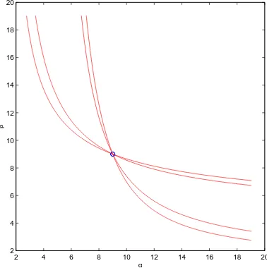
It is computed that, on the sphere kxk = 1, G has 6 extremal points, giv-ing four extremal values. By Theorem 4, to these extremal values,
cor-2 4 6 8 10 12 14 16 18 20 2
4 6 8 10 12 14 16 18 20
α
β
Figure 2: Fuˇc´ık curves for the problem (40), (41).
respond four Fuˇc´ık curves whose respective slopes, at the point (9,9), are
−2.6045,−2,−1/2, −0.3839. The four Fuˇc´ık curves are represented in Fig-ure 2. The curves of slopes −2,−1/2 come from solutions with u = v and are thus Fuˇc´ık curves for the problem
Their (well-known) equations are
6
Fuˇ
c´ık spectrum reduced to a curve in a
neighborhood of
(
λ
∗, λ
∗)
In this section, we discuss a situation where dim ker(L−λ∗A)>1,where the
nondegeneracy condition (15) of Theorem 1 fails to be satisfied, and which is nonetheless of practical interest. It concerns problems for which the following hypothesis is satisfied:
(H5) Forα, βclose toλ∗,ifc0(x∗, α, β) = 0 for somex∗ ∈ker(L−
λ∗A)\ {0}, then, for each x∈ker(L−λ∗A), c
0(x, α, β) = 0.
Such a condition holds for many periodic boundary value problems for au-tonomous differential equations. More precisely, the following result is pre-sented in [6] for scalar equations of order 2N (here,A =I).
Lemma 3. LetL: domL⊂L2((0,2π);R)→L2((0,2π);R)be a self-adjoint
linear ordinary differential operator of order 2N with constant coefficients, where
domL = {u∈H2N((0,2π);R)|
u(0) =u(2π), . . . , u(2N−1)(0) =u(2N−1)(2π)}.
If dim ker(L−λ∗I) = 2, then (H
4) holds.
When the operator L is self-adjoint, the matrix A diagonal and positive definite, and if (H5) holds, it follows immediately from the discussion of the
previous section that the sets F−,F+, defined by (35), (36), coincide and
that no other point of the Fuˇc´ık spectrum is contained in the set I ×I of Corollary 1. Hence, we have the following local uniqueness result.
Corollary 2. Let the hypotheses of Corollary 1 hold, as well as hypothesis (H5). Then, there is a unique Fuˇc´ık curve in the set I ×I; it crosses the
Example 1. The above corollary can be applied to the following system of
2nd-order ordinary differential equations:
u′′+k(u−v) +αu+−βu− = 0, (42)
v′′−k(u−v) +αv+−βv− = 0, (43)
considered with the periodic boundary conditions
u(0) =u(2π), u′(0) =u′(2π), v(0) =v(2π), v′(0) =v′(2π).
We take
L: domL⊂L2((0, π);R2)→L2((0, π);R2) : u
v
!
7→ − u
′′+k(u−v)
v′′−k(u−v)
!
,
domL being the set of functions in H2((0, π);R2) verifying the boundary
conditions; A will be the 2×2 identity matrix. The eigenvalues of L are of the form m2, or n2 −2k, m, n being integers. Provided that n2 −2k 6= m2 for all m, n ∈ N, all eigenvalues, except 0 and −2k, are of multiplicity 2.
The first system of eigenvalues then corresponds to solutions with u=v,the latter to solutions with u = −v. It is immediate that the nonlinear system (42), (43) has solutions with u = v, for which the Fuˇc´ık curves are easily computed; they intersect the diagonal at a point (m2, m2).The Fuˇc´ık curves
passing through the points (n2 −2k, n2 −2k) are more interesting. Using
arguments like the one used for the proof of Lemma 3, it can be shown that (H5) holds for the function c0 associated to such an eigenvalue. Hence, if
a Fuˇc´ık curve passes through the point (n2−2k, n2−2k), its slope at that
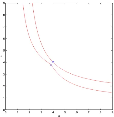
point must be equal to −1. We have represented in Figure 3, for k =−1.4, the Fuˇc´ık curves passing through the points (3.8,3.8) and (4,4) (obviously, in that figure, they are not restricted to the set I ×I of Corollary 2).
The situation is not so clear when L is not self-adjoint. Assuming that (H1) holds, we can make however, the following observation.
Proposition 1. Let (H1) hold. Assume that QA(ker(L−λ∗A)) = (Im(L−
λ∗A))⊥, and that
c0(x, α, β) = 0 =⇒c0(−x, α, β) = 0. (44)
If the sequence (αn, βn) ∈ Σ(L, A) is such that αn → λ∗, βn → λ∗, then
0 1 2 3 4 5 6 7 8 9 0
1 2 3 4 5 6 7 8 9
α
β
Figure 3: Fuˇc´ık curves for the problem (42), (43).
In other words, under (44), if a Fuˇc´ık curve passes through the point (λ∗, λ∗), its slope at that point must be equal to−1. Notice that the above
proposition uses much weaker assumptions that Corollary 2.
Proof. Using arguments as in the last part of Theorem 1, we claim that there must exist x∗ ∈ker(L−λ∗A), x∗ 6= 0 and a number η∗ such that
QA(|x∗|) +η∗QA(x∗) = 0.
By (44), we can replace x∗ by −x∗ in the above equation, which implies
η∗QA(x∗) = 0. Since QA is a bijection between ker(L−λ∗A) and (Im(L−
λ∗A))⊥, η∗ = 0 and the conclusion follows.
References
[1] K. Ben-Naoum, C. Fabry, D. Smets, Structure of the Fuˇc´ık spectrum and existence of solutions for equations with asymmetric nonlinearities, to appear in Proc. Roy. Soc. Edinburgh Sect. A.
[3] N.P. Cac, On nontrivial solutions of a Dirichlet problem whose jumping nonlinearity crosses a multiple eigenvalue, J. Differential Equations 80 (1989), 379-404.
[4] J. Campos, E.N. Dancer, On the resonance set in a fourth order equation with jumping nonlinearity, preprint.
[5] E. Dancer, On the Dirichlet problem for weakly nonlinear elliptic partial differential equations, Proc. Roy. Soc. Edinburgh Sect. A, 76A, (1977), 283-300.
[6] C. Fabry, Inequalities verified by asymmetric nonlinear operators, Non-linear Anal. TMA 33 (1998), 121-137.
[7] S. Fuˇc´ık, Boundary value problems with jumping nonlinearities, ˇCasopis Pest. Mat. 101 (1976), 69-87.
[8] S. Fuˇc´ık, A. Kufner, Nonlinear Differential Equations, Elsevier Science, The Netherlands, 1980.
[9] Th. Gallou¨et, O. Kavian, Resonance for jumping non-linearities, Com-mun. Partial Differ. Equations 7 (1982), 325-342 .
[10] M. Gaudenzi, P. Habets, Fuˇc´ık spectrum for a third order equation, J. Differential Equations 128 (1996), 556-595.
[11] J.V.A Gon¸calves, C.A. Magalh˜aes, Semilinear elliptic problems with crossing of the singular set, Trabalhos de Matem´atica n◦ 263, Univ. de Brasilia (1992), 23 pp.
[12] P. Krejˇc´ı, On solvability of equations of the 4th order with jumping
nonlinearities, ˇCasopis Pest. Mat., 108 (1983), 29-39.
[13] C.A. Magalh˜aes, Semilinear elliptic problem with crossing of multiple eigenvalues, Comm. Partial Differ. Equations, 15 (1990), 1265-1292.
[14] P.J. Pope, Solvability of non self-adjoint and higher order differential equations with jumping nonlinearities, PhD Thesis, University of New England, Australia, 1984.
[16] M. Schechter, Resonance problems with respect to the Fuˇc´ık spectrum, Preprint Univ. of California, Irvine, #960207, 1996.