Open/Closed String Topology and Moduli Space
Actions via Open/Closed Hochschild Actions
⋆Ralph M. KAUFMANN
Department of Mathematics, Purdue University, 150 N. University St., West Lafayette, IN 47907-2067, USA
E-mail: [email protected]
URL: http://www.math.purdue.edu/∼rkaufman/
Received October 30, 2009, in final form April 10, 2010; Published online April 30, 2010 doi:10.3842/SIGMA.2010.036
Abstract. In this paper we extend our correlation functions to the open/closed case. This gives rise to actions of an open/closed version of the Sullivan PROP as well as an action of the relevant moduli space. There are several unexpected structures and conditions that arise in this extension which are forced upon us by considering the open sector. For string topology type operations, one cannot just consider graphs, but has to take punctures into account and one has to restrict the underlying Frobenius algebras. In the moduli space, one first has to pass to a smaller moduli space which is closed under open/closed duality and then consider covers in order to account for the punctures.
Key words: string topology; Hochschild complex; double sided bar complex; foliations; open/closed field theory; moduli spaces; clusters of points
2010 Mathematics Subject Classification: 55P48; 81T30; 57R30; 16E40; 55P50
1
Introduction
There has been a lot of interest in studying open/closed theories from physics and mathematics. In physics this goes back to boundary CFTs and D-branes with an extensive literature. In mathematics motivation come from open/closed string topology, Gromov–Witten invariants and TQFT again with a virtual onslaught of ideas. Sources relevant to our constructions are [3, 18, 19, 20]. In this spirit, there have been many interesting forays into the subject of open/closed operations [21,4,1,5,2].
Our point of view comes from the geometry provided in [11, 7] and the operations on Hochschild complexes defined in [8] via correlations functions. In this paper, we extend these correlation functions to the open/closed case. This leads to a dg-action of a Sullivan-type PROP yielding string topology type operations and a cell level moduli space action on Hochschild com-plexes. There are several surprising details and conditions which to our knowledge have not been fully discussed previously. These obstacles make the passage from the closed case to the open/closed case far from being evident.
The first is that – unlike the closed case – in the open/closed case, the role of punctures cannot be suppressed, as they can arise as the result of an open gluing. These punctures contribute new factors to the correlators. Another consequence of the presence of punctures is that in the moduli space case the underlying ribbon graph needs extra decorations marking possible punctures and one cannot define the string topology type operations just by looking at open/closed graphs of Sullivan type. One has to know the puncture structure inside the complementary regions as well.
⋆This paper is a contribution to the Proceedings of the XVIIIth International Colloquium on Integrable
Sys-tems and Quantum Symmetries (June 18–20, 2009, Prague, Czech Republic). The full collection is available at
Secondly we need a compatibility equation for the dg-PROP to operate, which is satisfied if the coefficient modules of the Hochschild complexes have a geometric origin. A further unexpected detail is that the moduli space is not the first moduli space one would choose. For each moduli space one has to pick out a subspace that satisfies open/closed duality and then consider covers or rather spaces which are stratified by covers of the usual moduli spaces. These are brane labelled open/closed moduli spaces c/oMs,β
g,δ1,...,δn of bordered surfaces with punctures
on the boundary and clusters of marked points on the interior. The main results are
Theorem 1. There is an open/closed colored β brane labelled c/o dg-PROP cell model of the open/closed colored brane labelled topolgical quasi PROP(see AppendixA.7)Sullgc/o which acts in a brane labelled open/closed colored dg-PROP fashion on the brane labelled Hochschild complexes for a β-Frobenius algebra which satisfies the Euler condition(E); see Definition 4.5.
This theorem defines open/closed string topology type actions for compact manifolds that are simply connected.
Theorem 2. There is an operadic cell model associated to the β-brane labelled open/closed mo-duli spaces c/oMs,βg,δ1,...,δn which acts on β-labelled Hochschild co-chains via operadic correlation functions with values in a β-labelled Hom operad.
The actions in both cases are made possible by a discrete version of the c/o action.
Theorem 3. For a basicB-Frobenius algebra the c/o structure of discretely weighted arc-graphs acts on he collection of complexes B(β) and the isomorphic Hochschild complexes via the corre-lation functions Y defined by equations (4) and (5).
The restriction basic B-Frobenius algebras is simply of expository nature. We can deal with general systems of B-Frobenius algebras. For this we would introduce a new propagator formalism which we will do elsewhere as not to put even more technical structures into this exposition.
We begin by reviewing the relevant structures from [11] in Section 2. We then go on to construct the relevant spaces which carry the topological structures. The first of these is taken from [11] and is concerned with graphs on windowed surfaces. We define a generalization and a restriction of this structure. The restriction is the space that yields moduli spaces of curves with marked points and tangent vectors, while the extension is used to define the open/closed Sullivan PROP. We also briefly discuss the moduli spacec/oMs,βg,δ1,...,δn which provides the chain
models for the moduli space action. In all these cases, we associate a chain complex to these spaces where each basis element, or cell, is indexed by a graph of arcs on the given windowed surface.
In Section 3, we review the open/closed gluing operations in the geometrical setting. The algebraic counterpart is given by brane labelled bar complexes of brane labelled systems of Frobenius algebras which we introduce in Section4.
2
Review of the KP-model for open/closed strings
We recall the main features of the KP-model for open/closed string interactions via foliations [11]. The interactions are given by surfaces with boundary and punctures together with a foliation. There are marked points on the boundary (at least one per boundary) and possibly also marked points in the surface. The part of the boundary between two marked points is called a window. The foliation is thought of as being transverse to the propagating string and as keeping track of splitting and recombining of pieces of string. The foliation and its partial transverse measure are encoded in a graph of weighted arcs. Furthermore there is the data of a brane labelling which keeps track of the branes that the strings might end on.
Given two windows, either on two disjoint surfaces or on the same surface, we can glue them and the foliations together if their weights agree on these windows. In [11] we showed that this gluing gives rise to an c/o structure on the topological level and induces chain level operations, which descend to a bi-modular operad on the homology level.
More technically, the setup is as follows:
2.1 Arc graphs in brane labelled windowed surfaces
A windowed surface F =Fgs(δ1, . . . , δr) is a smooth oriented surface of genus g≥0 with s≥0
punctures andr≥1 boundary components together with the specification of a non-empty finite subset δi of each boundary component, for i= 1, . . . , r, and we let δ =δ1∪ · · · ∪δr denote the
set of all distinguished points in the boundary∂F ofF and letσ denote the set of all punctures. The set of components of ∂F −δ is called the setW of windows.
Furthermore one needs to specify a brane labellingβ. For this we first fix a set B of basic brane labels and denote by P(B) power set. Notice that ∅∈ P(B), this will encode the closed
sector. The elements ofP(B) of cardinality bigger than one should be thought of as intersecting branes. These give room for extra data, but it is possible to set all the contributions for these “higher intersection” branes to zero in a given model.
Abrane-labeling on a windowed surfaceF is a function
β : δaσ→ P(B),
where ⊔ denotes the disjoint union, so that if β(p) = ∅ for some p ∈ δ, then p is the unique
point of δ in its component of∂F. A brane-labeling may take the value∅at a puncture.
A windoww∈W on a windowed surfaceF brane-labeled byβ is calledclosedif the endpoints of w coincide at the point p ∈δ and β(p) = ∅; otherwise, the window w is called open. Each
window defines a pair of brane labels β(w) which is the pair (S, T) of the brane labels of the beginning and end of the window (these may coincide).
2.1.1 Arc families
We define the sets
δ(β) ={p∈δ :β(p)6=∅}, σ(β) ={p∈σ :β(p)6=∅}.
Define aβ-arcainF to be an arc properly embedded inF with its endpoints inW so thata is not homotopic, fixing its endpoints, to ∂F −δ(β). For example, given a distinguished point p ∈ ∂F, consider the arc lying in a small neighborhood that simply connects one side of p to another inF;ais aβ-arc if and only ifβ(p)6=∅. We will call such an arc asmall arcaroundp.
Given a positively weighted arc family inF, let us furthermore say that a window w ∈ W is active if there is an arc in the family with an endpoint in w, and otherwise the window is inactive.
2.1.2 The mapping class group and arc graphs
The (pure) mapping class groupM C(F) ofF is the group of orientation-preserving homeomor-phisms of F pointwise fixingδ∪σ modulo homotopies pointwise fixing δ∪σ.
M C(F) acts naturally on the set of β-arc families. An arc graph is an equivalence graph under this action.
2.2 Arc spaces, moduli spaces and the open/closed Sullivan PROP
2.2.1 The Arc spaces
A weighting on an arc family is the assignment of a positive real number to each of its compo-nents. A weighting naturally passes to the arc graph. A weighting is called discrete if it takes values in N.
Let Arc′(F, β) denote the geometric realization of the partially ordered set of allβ-arc families in F. Arc′(F, β) is described as the set of all projective positively weighted β-arc families in F with the natural topology. (See for instance [12] or [15] for further detail.)
M C(F) again acts naturally on Arc′(F, β). The arc complex is defined to be the quotient under this action
Arc(F, β) = Arc′(F, β)/M C(F).
We shall also consider the corresponding deprojectivized versions: Arcg′(F, β)≈Arc′(F, β)×
R>0 is the space of all positively weighted arc families inF with the natural topology, and
g
Arc(F, β) =Arcg′(F, β)/M C(F)≈Arc(F, β)×R>0.
For any windowed surfaceF, define
g
Arc(F) =GArc(g F, β),
where the disjoint union is over all brane-labellings onF.
g
Arc(n, m) =G α∈Arc(g F) : α has nclosed andm open active windows and no inactive windows
,
where the disjoint union is over all orientation-preserving homeomorphism classes of windowed surfaces.
2.3 The open/closed Sullivan spaces
As proved in [11], the spacesArc(g n, m) form an c/o structure, see the appendix for the complete definition. We will now construct a suitable PROP to capture string topology type operations. First, we have to add additional data to the surface (F, β), which is a partitioning i/o := {Win, Wout} of all of the windows of F into “in” and “out” windows. A β-arc family (or arc
graph) on such a surface is called of Sullivan typeif
We set Sullc/o′(F, β,i/o) the geometric realization of the partially ordered set of all β-arc
families of Sullivan type. And letSullc/o(F, β,i/o) be the quotient under the action ofM C(F). As above, we also consider the deprojectivized versions Sullgc/o(F, β,i/o)
g
Sullc/o(F) =GSullgc/o(F, β,i/o),
where the disjoint union is over all brane-labellings onF and partitions i/o.
g
Sullc/o(n1, n2, m1, m2) =
G(
α∈ Sullc/o(F) :
α hasn=n1+n2 closed and m=m1+m2 open
windows with n1 and m1 active closed resp. open “in”
windows and n2,m2 closed resp. open “out” windows
,
where the disjoint union is over all orientation-preserving homeomorphism classes of windowed surfaces.
Notice that Sullgc/o(n, m) is also graded by the number k of inactive “out” windows – by definition all “in” windows are active.
2.4 Moduli space
The spaces ofβ arc families contains a moduli space. We call an arc family or graphquasi-filling, if all complementary regions are polygons or once punctured polygons.
The weighted quasi-filling graphs form a subspace of each Arc(F, β) which is homeomorphic to the moduli spaces Msg,t1,...,tn, of genus g surfaces with n+s marked points, where for the
first n marked points ti ≥ 1 tangent vectors at the ith marked point are specified. This is
independent of β since the small arcs only thicken the moduli spaces by a factor of R>0. This
fact is straightforward using the dual graph and Strebel differentials [17].
2.4.1 Open/closed duality moduli space of open/closed brane labelled surfaces
with marked point clusters
The moduli space Msg,t1,...,tn, is actually too small and too big for its cell model to act, as we
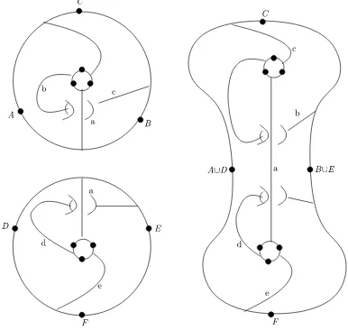
will discuss below. It is too big in the sense that there are gluings which when allowing open windows on boundaries unexpectedly take us out of moduli space on the chain level; see Figs.7 and 8. There is however a subspace of this space given by the arc families that are in general position with respect to the open/closed duality (see Fig. 9) which solves this problem. The other problem that arises which is unique to the open sector is that unlike in [7,8] we cannot restrict to the case of no punctures;s= 0. But gluing with internal punctures is again not stable in the moduli space case. This problem is overcome by introducing clusters of brane labelled points. The resulting space is the open/closed duality moduli space of open/closed brane labelled surfaces with marked point clustersc/oMs,βg,δ1,...,δn. The details are given in Section7 below.
3
Geometric c/o structures
points. When we glueβ arc families, we glue the surfaces and glue the arc families as foliations. We will now review this process according to [11].
3.1 The gluing underlying the topological c/o structure
If α ∈ Arc(g n, m), then define the α-weight α(w) of an active window w to be the sum of the weights of arcs inαwith endpoints inw, where we count with multiplicity (so if an arc inα has both endpoints in w, then the weight of this arc contributes twice to the weight ofw).
Suppose we have a pair of arc families α1, α2 in respective windowed surfaces F1, F2 and
a pair of active windows w1 in F1 and w2 in F2, so that the α1-weight of w1 agrees with the α2-weight of w2. Since F1, F2 are oriented surfaces, so are the windows w1, w2 oriented. In
each operation, we identify windows reversing orientation, and we identify certain distinguished points.
To define the open and closed gluing (F1 6=F2) and self-gluing (F1=F2) ofα1,α2 along the
windowsw1,w2, we identify windows and distinguished points in the natural way and combine
foliations.
A crucial difference between the closed and open string operations is that in the closed case, the points are thought of as marked, which in the open case the points behave like punctures. This means that in the closed case, we replace the distinguished point by simply forgetting that is was distinguished. This way no puncture is created. In the open case the distinguished points always give rise to other distinguished points or perhaps punctures. In any case whenever distinguished points are identified, one takes the union of brane labels (the intersection of branes) at the new resulting distinguished point or puncture.
3.1.1 Closed gluing and self-gluing
Identify the two corresponding boundary components of F1 and F2, identifying also the
distin-guished points on them and then including this point in the resulting surface F3. F3 inherits
a brane-labeling from those on F1, F2 in the natural way. We furthermore glue α1 and α2
together in the natural way, where the two collections of foliated rectangles in F1 andF2 which
meetw1 and w2 have the same total width by hypothesis and therefore glue together naturally
to provide a measured foliation F of a closed subsurface ofF3.
3.1.2 Open gluing
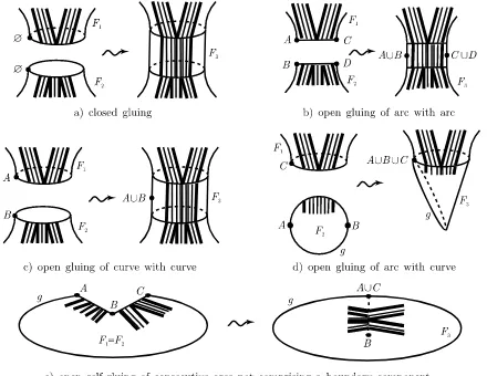
The surfaces F1 and F2 are distinct, and we identify w1 tow2 to produce F3. There are cases
depending upon whether the closure of w1 and w2 is an interval or a circle. The salient cases
are illustrated in Fig. 1, b–d. In each case, distinguished points on the boundary in F1 and F2
are identified to produce a new distinguished boundary point in F3, and the brane labels are
combined, as is also illustrated. As before, since theα1-weight onw1 agrees with theα2-weight
on w2, the foliated rectangles again combine to provide a measured foliation F of a closed
subsurface of F3.
Open self-gluing.There are again cases depending upon whether the closure ofw1 orw2 is
a circle or an interval, but there is a further case as well when the two intervals lie in a common boundary component and are consecutive. Other than this last case, the construction is identical to those illustrated in Fig. 1, b–d. In case the two windows are consecutive along a common boundary component, again they are identified so as to produce a surface F3 with a puncture
Figure 1. The different cases of gluing.
At this stage, we have only constructed a measured foliationF of a closed subsurface ofF3,
and indeed, F will typically not be a weighted arc family, but the sub-foliationF′ comprised of leaves that meet ∂F corresponds to a weighted arc familyα3 inF3. Notice that theα3-weight
of any window uninvolved in the operation agrees with itsα1- orα2-weight.
The assignment ofα3 in F3 to αi in Fi, for i= 1,2 completes the definition of the various
operations. Associativity and equivariance for bijections are immediate, and so we have our first non-trivial example of a c/o structure; see AppendixA for the precise definition.
3.2 Extended gluing and the open/closed Sullivan PROP
Remark 3.1. We do not wish to formalize c/o PROP structures here. A PROP gluing is given by pairing of all “ins” to all “outs” of two different surfaces and gluing on all of them. In apparent terminology, we can have the open and closed PROP substructures separate or at once. Technically there are also so-called vertical compositions which in our cases are always just disjoint unions. The brane labelling is handled in the same fashion as in the c/o case. For more details see Appendix A.7.1.
Proposition 3.2. The open/closed Sullivan spaces are closed under the extended gluing, when gluing an open (respectively closed) “in” to an open (respectively closed) “out” window with the same weight or to an empty “out” window.
Corollary 3.3. This also gives the structure of a c/o, i/o modular operad in the terminology of the appendix. This implies that these spaces form c/o PROP. These structures also exist in the brane labelled case.
Proof . Both conditions for families in the Sullivan spaces are stable under the gluing. (1) If arcs only run from “in” to “out”, they also do so after gluing an “in” to an “out” window: Indeed a foliation could only run from “in” to “in” on the glued surface if there was a foliation running from “in” to “in” in the surface to whose “in” window we glue. The extended gluing only kills foliations. (2) After gluing all “in” boundaries are active: This is clear if we do not glue to an empty “out”. But even if we glue to an empty “out” this holds true, since in this case only leaves get deleted on the surface to whose “in” we glue. These foliations run to “out” windows of that surface and hence to “out” windows of the glued surface. The “in” windows of the glued surface are unaffected. The number of inactive “out” windows may of course increase. Since the gluing is associative, we can obtain a c/o PROP gluing by simply gluing successively as described in the appendix. The first gluing will be a non-self gluing, while all remaining gluings are self-gluings. Since gluing is associative this is insensitive to the order chosen.
The brane labelling is external to the foliation gluing, so the last statement readily follows.
There is actually a open/closed colored dg-PROP structure on the chain level, if we use cellular chains as we demonstrate in Section 6. This is induced by a topological quasi-PROP structure on the topological level; see the appendix for the definitions of these types of PROPs.
3.3 Discretization of the model N-valued foliations
We wish to point out that the subset of discrete valued foliations is stable under the compositions in both the c/o structure and the c/o PROP structure.
3.3.1 Discrete representation for discretely weighted β-arc families
In order to decorate, we will change the picture slightly. Previously we had arc graphs, whose edges are not allowed to be parallel. For adiscretely weightedβ-arc families with weightingwtwe will consider its leaf representationto be the foliation each of whose bands ehas wt(e) number of leaves. This means that we consider an new type of arc graph which has wt(e) parallel edges for each underlying edge of the original arc graph. We will call this the discrete representative of the arc graph.
4
Algebraic c/o structures
Given a β-arc graph with weights that are natural numbers, we are going to associate an op-eration on the Hochschild complexes CH∗(A∅, MB,B′) of a fixed Frobenius algebra A
∅ with
of Frobenius algebras AB indexed by elements ofB: MB,B′ :AB′ ⊗AB. These operations will
be defined on the isomorphic double sided bar-complexesB(AB, A∅, AB′). For most operations
we will need thatA∅is commutative, but this is not always the case. We will indicate when the commutativity can be dropped.
4.1 Frobenius algebras and systems of Frobenius algebras
4.1.1 Notation for Frobenius algebras
The main actors are Frobenius algebras, so we will fix some notation.
Recall that a Frobenius algebra (FA) is a triple (A,1,h, i) where (A,1) is a unital (super-) algebra andh, i is a non-degenerate (super-) symmetric even pairing which satisfies
hab, ci=ha, bci.
We will set
Z
a:=ha,1i.
Then R is cyclically (super-)invariant, i.e. a trace
Z
abc=hab, ci=hc, abi=
Z
cab.
Sinceh, i is non-degenerate onA, so ish, iA⊗A:=h, i ⊗ h, i ◦τ2,3 onA⊗2⊗A⊗2. Hereτ2,3
is the commutativity constraint for the symmetric monoidal category applied to the second and third factors, be it the category of vector spaces, dg-vector spaces orZ/2Zgraded vector spaces
In our current setup this just interchanges the second and third factors ofA⊗A⊗A⊗A or in the super case changes these factors and introduces the usual super sign.
We will omit all super signs from our discussion as they can be added in a straightforward fashion.
The multiplicationµ:A⊗A→Ahas an adjoint ∆ :A→A×A defined by
h∆a, b⊗ciA⊗A=ha, bci. (1)
Moreover given a FA we will consider a basis ∆i, setgij =h∆i,∆jiand letgij the coefficients
of the inverse of (gij), viz. the inverse “metric”.
There are two special elements
e=µ∆(1) =X
ij
∆igij∆j,
which we call the Euler element and
C = ∆(1) =X∆igij⊗∆j,
which we call the Casimir element.
Notice that Euler element commutes with every element.
ae=aµ∆(1) =µ∆(a) =µ∆(1)a=ea.
This follows by direct computation and the Frobenius relations
(id⊗µ)(∆⊗id) = ∆µ= (µ⊗id)(id⊗∆),
4.1.2 Adjoint maps
Notice that for any map r : A → B between two Frobenius algebras there is an adjoint map r†:B →A defined by
hr†(b), ai=hb, r(a)i.
This is equivalent to
Z
r†(b)a=
Z
br(a). (2)
These maps arise in geometric situations as follows. Let i: N → M be the inclusion map, whereM is a compact manifold andN is a compact submanifold. Theniinduces a mapi∗from A :=H∗(M) to B :=H∗(N). By Poincar´e duality there is a push forwardi∗ :B → A. In the previous notation if r=i∗ thenr†=i∗.
Lemma 4.1. In general, we have the Projection Formula
r†(r(a)b) =ar†(b).
Proof .
hr†(r(a)b), ci=hr(a)b, r(c)i=hb, r(ca)i=har†(b), ci,
where we used the cyclic symmetry of the product twice.
With the self-intersection condition Section4.6in mind, we define the element
e⊥r :=r(r†(1)).
4.1.3 Systems of Frobenius algebras
Definition 4.2. AB-Frobenius algebra is a set of Frobenius algebrasAS indexed byS∈ P(B)
together with algebra maps rS,S′ : AS → A′
S whenever S ⊂ S′, such that for S ⊂ S′ ⊂ S′′:
rS′,S′′◦rS,S′ =rS,S′′.
Note that in particular if A∅ is commutative every AS is an A∅module via the restriction
map. More precisely, everyAS is a left and a rightA∅module via the mapsλ(a, a′) :=r∅S(a)a′
and ρ(a, a′) := a′r
∅S(a). If A∅ is not commutative, we still have that AS is a left A∅module
and a rightAop∅ module.
4.1.4 Basic brane label systems
Given a brane label set B one set choices of B-Frobenius algebras is given by a collection AB,
B ∈ B and A∅together with maps rB :A∅→AB.
For any S ∈ PB with |S| ≥2 we simply set AS = 0 where we allow the zero algebra to be
a Frobenius algebra.
We call these systems basic brane label systems and for simplicity deal only with these. The data of the Frobenius algebras and morphisms will be called a basicB Frobenius algebra.
Notation 4.4. Given AB we will use the notation 1B, eB, ∆Bi , h, iB, gijB, g ij
B, e⊥B, . . . for its
unit, Euler element, basisAB, metric inverse metric,e⊥rB etc.
We will also omit the label∅ i.e. writeefore∅,A forA∅if no confusion can arise.
Definition 4.5. We say that a basicB-FA satisfies the condition of commutativity (C) if A∅ is commutative.
And we say that aB-FA satisfies the the Euler compatibility condition or thecondition (E) if for all B ∈ B,a(1), a(2) ∈AB
(E) X
ij
r†B a(1)∆Bi gijBrB† ∆Bi a(2)=e∅r†B a(1)a(2).
Definition 4.6. A basic B-Frobenius algebra satisfies the self-intersection condition (I) if for all B ∈ B
(I1) rBrB†(a) =ae⊥B and (I2) eBe⊥B=rB(e).
Proposition 4.7. A basic system of B Frobenius algebra which satisfies the self-intersection condition (I) satisfies the Euler condition(E).
Proof . We will show that the r.h.s. and the l.h.s. of (E) have the same inner product with any element bof A:
where the first equality follows from equation (2), the third equality from the definition ofeB
and the fact thateB as the Euler element commutes with all other elements and the last equality
follows from the projection formula and the fact thatecommutes.
4.1.5 Geometric data
One example of the basic data is given by a compact manifold M together with a collection NB ⊂ M, B ∈ B of compact submanifolds. We can then set AB := H∗(NB) and use the
restriction maps rB given by pullback. These satisfy the first condition (I1) of (I) due to the
self-intersection formula where e⊥
B = e(NM/NB) is the Euler class of the normal bundle of NB
inM. The second condition (I2) follows from the excess intersection formula for homology [16]
applied to the diagram
Alternatively one can use decompositionT M|NB = T NB⊕NM/N B and multiplicativity of
Remark 4.8. We can also formalize the geometricity by staying in the framework of Frobenius algebras, but postulating a new axiom which guarantees the equations one would obtain from excess intersection formulas from all embedding and intersection diagrams analogous to (3).
Corollary 4.9. A basic geometricB Frobenius algebra satisfies the Euler condition (E).
4.1.6 Hochschild complexes
The action on the closed sector is on the Hochschild cochain-complex of A. Recall that the Hochschild chain complex of an Abimodule M is the complex CHn(A, M)
CHn(A, M) =M ⊗A⊗n
and whose differential is given byd=Pi(−1)id
i, where thediare the pre-simplicial differentials
d0(m⊗a1⊗ · · · ⊗an) =ma1⊗a2⊗ · · · ⊗an,
di(m⊗a1⊗ · · · ⊗an) =m⊗a1⊗ · · · ⊗ai−1⊗aiai+1⊗ai+2⊗ · · · ⊗an,
dn(m⊗a1⊗ · · · ⊗an) =anm⊗a1⊗ · · · ⊗an−1.
There are degeneracies inserting 1 into theith position
si: CHn(M, A)→CHn+1(M, A),
m⊗a1⊗ · · · ⊗an7→m⊗a1⊗ · · · ⊗ai−1⊗1⊗ai⊗ · · · ⊗an.
The Hochschild chain complex CH∗(A, M) is also sometimes called the cyclic bar complex and is denoted by B∗(A, A).
The Hochschild co-chain complex is dually given by
CHn(A, M) = Hom(A⊗n, M)
with the dual differential dCH∗ =Pi(−1)idCHi ∗,dCH∗ : CHn(A, M)→CHn+1(A, M), where for f ∈CHn(A, M)
dCH0 ∗f(a1⊗ · · · ⊗an+1) =a1f(a2⊗ · · · ⊗an),
dCHi ∗f(a1⊗ · · · ⊗an+1) =f(a1⊗ · · · ⊗ai−1⊗aiai+1⊗ai+2⊗ · · · ⊗an),
dCHn+1∗(a1⊗ · · · ⊗an+1) =f(a1⊗ · · · ⊗an)an+1.
The degeneracies dualize tosCH∗
i : CHn(A, M)→CHn−1(A, M)
sCHi ∗f(a1⊗ · · · ⊗an−1) =f(a1⊗ · · · ⊗ai−1⊗1⊗ai⊗ · · · ⊗an−1).
In caseM =A multiplication of functions gives a natural product
∪: CHn(A, A)⊗CHm(A, A)→CHn+m(A, A).
Notice that if A is a Frobenius algebra, it is isomorphic to its dual as a bi-module. Since A ≃ Aˇ, CHn(A, A) ≃ A⊗Aˇ⊗n ≃ A⊗n+1 ≃ CH
n(A, A). The cup product and the product
4.1.7 Reduced Hochschild complex
For technical reasons discussed in [8] it is actually easier to work with the reduced Hochschild co-chain complex CH∗(A, A). This complex is the subcomplex of functions that vanish on all degeneracies that is functionsf :A⊗n→Asuch thatf(a
1, . . . ,1, . . . , an) = 0 where 1 is plugged
in into any position. The complex inherits the differential and computes the same cohohmology as the original complex. Dually there is the reduced bar complex CH∗(A, A) or ¯B∗(A, A) which we shall use in the closed sector.
4.1.8 Double sided bar construction
For the open action, we will consider the double sided bar complexesB(S, T) :=B•(AS, A, AT)
whose components are defined as Bn(AS, A, AT) =AS⊗A⊗n⊗AT
and whose differential is given byd=Pi(−1)idi, where thediare the pre-simplicial differentials
d0(aS⊗a1⊗ · · · ⊗an⊗aT) =aSa1⊗a2⊗ · · · ⊗an⊗aT,
di(aS⊗a1⊗ · · · ⊗an⊗aT) =aS⊗a1⊗ · · · ⊗ai−1⊗aiai+1⊗ai+2⊗ · · · ⊗an⊗aT,
dn(aS⊗a1⊗ · · · ⊗an⊗aT) =aS⊗a1⊗ · · · ⊗an⊗anaT.
Remark 4.10. Notice that since we are dealing with Frobenius algebras, this is isomorphic to CH•(A, AT ⊗AS) and again the differentials dualize to one and another.
4.1.9 Degeneracies
The double sided complex is actually simplicial, which means that it also has degeneracy maps si: Bn(AS, A, AT)→Bn+1(AS, A, AT),
aS⊗a1⊗ · · · ⊗an⊗aT 7→aS⊗a1⊗ · · · ⊗ai−1⊗1⊗ai⊗ · · · ⊗an⊗aT.
4.1.10 Brane labelled bar complexes
Fix aB Frobenius algebra. For a windoww on a brane labelled surface with labellingβ we set B(w) :=B(β(w)) ifw is open and B(w) =B(β(w)) =B(∅,∅) := CHn(A, A) if w is closed.
4.2 Gluing in brane labelled complexes
As we have noted, the complexes B(β) have non-degenerate graded inner products which allows us to dualize them. Using this dualization, we can compose two correlation functions for the basic brane label case. In the general case we would need to introduce propagators to do this. We will refrain from adding this technical point here for clarity of the discussion.
Given (graded) vector spaces Vβ : β ∈ I over a ground field k with an involution ¯ on I,
j be the Casimir element for the induced pairing between Vβ
and Vβ¯ expressed in a basis (∆βi).
where Land L′ are labelling sets by inserting a Casimir.
=X
ij
Y O
l∈L\{l0} vl
⊗∆βi
gijY′ O
l′∈L′\{l′
0} vl′
⊗∆¯βj
,
where ∆βi is in the positionl0 and ¯∆βj is in positionl′0. Ifβl0 6= ¯βl′0 we set the composition to 0. In the more general case these would be non-zero and the composition would use propagators.
Alternatively, we could also dualize the mapsY using Cβl in any position l to obtain maps
toVβl instead ofkand then compose these maps. There is an analogous procedure for self-gluing.
Remark 4.11. In our case I =B × B ∪ {∅,∅}, (S, T) = (T, S),Vβ =B(β) the corresponding
bar complex and the isomorphisms¯:B(S, T)→B(T, S) are given by
aS⊗a1⊗ · · · ⊗an⊗aT 7→aT ⊗an⊗ · · · ⊗a1⊗aS
and B(∅,∅)→B(∅,∅)
a0⊗ · · · ⊗an7→a0⊗an⊗ · · · ⊗a1.
Remark 4.12. In order to give a brane labelled c/o structure, we should consider slightly enriched more complicated data. For this we would have to look at tensors products of cyclic tensor products of bar complexes B(S1, S2)⊗B(S2, S3)⊗ · · · ⊗B(Sn, S1). Again in the interest
of brevity, we will not introduce this kind of complexity in a formal fashion here.
Remark 4.13. There are actually two c/o structures, one can compose the bar complexes or their duals, viz. the correlators. Of course these operations are dual to each other.
5
Correlators
5.1 A universal formula for correlators
There is a universal formula for the correlators. It is given by partitioning, decorating and decomposing the surface of a discretely weighted arc family along the arcs into little pieces of surfaceSi and integrating around these pieces. We will now give the details.
5.1.1 Decorating the boundary
Fix a basic B collection of Frobenius algebras. For eachdiscretely weighted β-arc family α, we will define a map
Y(α) := O
w∈Windows of α
B(β(w))→k.
These functions are homogeneous and their homogeneous components are zero by definition unless aw ∈Bα(w)−1(β(w)).
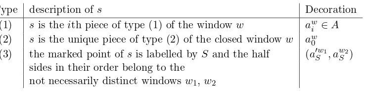
Given a collection of homogeneous elements we will decorate the pieces belonging to the boundary of the discrete representation of α by the elements of the bar complexes
aw =awS ⊗aw1 ⊗ · · · ⊗awα(w)−1⊗a′Tw if β(w) = (S, T),
aw =aw0 ⊗aw1 ⊗ · · · ⊗awα(w)−1 if β(w) = (∅,∅).
(1) those not containing a marked point,
(2) those containing a marked pointβ-labelled by ∅,
(3) those containing a marked point withβ-label not∅.
In case (3), if we remove the marked point we will have two components which we will call half sides of the boundary piece. Now each piece of type (1) and the half sides of the pieces of type (3) belong to a unique window. A piece of type (2) comes from a unique closed window/boundary component. Moreover these pieces all come in a natural linear order in each window as do the half sides of a piece of type (3) if we consider the marked point to lie in between the half sides.
We decorate the boundary pieces as follows:
Type description of s Decoration
sides in their order belong to the not necessarily distinct windows w1,w2
5.1.2 Weights
Let {Si : i ∈ I} be the components of complement of the discrete representative of a given
discretely weighted β arc family α. Each of these pieces has a polygonal boundary, where the sides of the polygons alternate between pieces of the boundary and arcs running between them. If we decorate the surface as described above every second side is a decorated piece of boundary. We will call these the decorated sides.
To each decorated sidesofSi, we associate a weight dependingωon its type and decoration.
Table 1. General weights.
Type Decoration Weight ω(s)
(1) swithout marked point a∈A∅ a
Moreover, the Si are oriented and so hence are their boundaries. This means that the sides
comprising each boundary component come with a cyclic order. If there is only one boundary component for a givenSi, this gives a cyclic order over which we will integrate the given weights.
5.1.4 Signs
The correlators above actually have hidden signs which come from the permutation of the input variables to their respective position. In the bar complexes these signs can be read off by imposing that the tensor symbols have degree 1. On the geometric side there are signs as well which are fixed by fixing an enumeration of the flags, angles or edges. In general we adhere to the sign conventions spelled out in [8, Section 1.3.4].
5.2 Action of the c/o structure of discretely weighted arc-graphs
We say a c/o structure acts via correlation functions if the composition of the elements of the c/o is compatible with the composition of the correlation functions. In short Y(α◦w,w′ α′) = Y(α)◦w,w′ Y(α′) where ◦w,w′ denotes the gluing of the window w and w′ holds as well as the
corresponding equation for the self-gluing.
Theorem 5.1. For a basic B-Frobenius algebra the c/o structure of discretely weighted arc-graphs acts on the collection of complexes B(β) and the isomorphic Hochschild complexes via the correlation functions Y.
Just like there are algebras over operads, we can define algebras over c/o structures. The theorem above reads: The collection of bar complexes B(S, T) form an algebra over the c/o structure of discretely weighted arc-graphs.
Proof . The proof is a case by case study which occupies Section 5.3.
5.3 Case by case analysis of the discrete arc-graph action
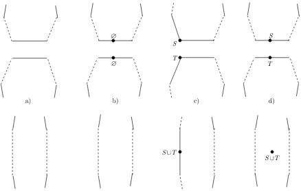
The gluing of the surfaces with discrete arcs breaks down into individual local gluings of pairs of surfaces Si and Sj′. In case the surfaces are distinct, there are five cases of this gluing depicted
in Figs.2and3. The cases a) and b) are the ones familiar from the closed gluing [8], the cases c) and d) are new in the open/closed case. The gluing c) appears when we are gluing two open windows where none of them is the only window in its boundary component. The gluing d) appears when gluing two open windows each of which is the only window in its boundary component. The most complicated case is when one of the windows is the only window, while the other is not. This case e) is given in Fig. 3.
5.3.1 Non-self gluing, the closed case
In the case that there is no self-gluing: a)–b) correspond to:
Z
where the w, w′, w′′ are the weights of the adjacent sides and we use Einstein summation conventions. We have also included any factors of einto the ellipses.
5.3.2 Non-self gluing case in the simple brane case
Assuming the simple brane case, all labels have to be the same, say S then c) corresponds to
Figure 2. Types of local gluings: a) two sides without marked points; b) side with marked point labelled by∅to side with marked point labelled by∅; c) half a labelled side with marked point labelled byS to
half side with marked point labelled byT; d) full side with labelled point marked byS to full side with labelled point marked byT.
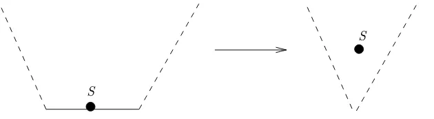
Figure 3. e) Gluing of a lone window with an open marked point to window with two marked points.
=
Z
w′. . . wrS†(aSa′S)w′′′. . . w′′=
Z
. . . wr†S(aSaS′ )w′′′. . . w′′w′,
while d) corresponds to
Z
. . . wr†S(∆Si∆Sk)w′. . .
gijSgSkl
Z
. . . w′′r†S(∆Sl∆Sj)w′′′. . .
=
Z
w′. . . wrS†(∆Si gSij∆Sj)w′′′. . . w′′=
Z
. . . wr†S(eS)w′′′. . . w′′w′.
The case e) has two subcases. 1) there are three surfaces which are glued:
Z
. . . wrS†(aS∆Si)w′. . .
gSij
Z
. . . w′′rS†(∆Ska′S)w′′′. . .
gklS
Z
. . . w(vi)r†S(∆Sj∆Sl)w(v). . .
×
Z
S
a′SrS(w′′′. . . w′′)∆Sk
gSkl
Z
S
∆SlrS w(v). . . w(vi)∆SjgijS
Z
S
∆SirS(w′. . . w)aS
=
Z
S
. . . wr†S(aSa′S)w′′′. . . w′′w(v). . . w(vi)w′,
and the case 2) where only two surfaces are glued
Z
In this case we have to use commutativity (C) and the Euler compatibility (E):
gSij
which is the contribution we get from the glued surfaces, since there is one self-gluing involved and this makes the Euler characteristic go up by one.
5.3.3 The self gluing cases
So far we have assumed that the two (half) sides that are glued are on different Si and Sj′. It
can happen that they belong to the same surface. In these cases, much like in the case e) 2), there are fewer integrals and instead an Euler class factor e appears. In the case that there is self-gluing: a)–b) correspond to:
This r.h.s. is the contribution to correlator for the glued surface since the self-gluing changes the Euler characteristic by −1. Again we need to use (C).
The cases c), d) are analogous to the case e) 2). The self gluing decreases the Euler charac-teristic by one, while the summation gives the factor eby condition (E). The two cases for e) then either involve only one or two integrals, respectively; correspondingly the gluing then gives rise to a factor of eore2, respectively.
There is one more local gluing which comes from gluing consecutive windows corresponding to Fig.1 cases e) and f). In these cases two half sides of asingleside marked by a point labelled by some S 6=∅are glued together.
This corresponds to the following equation in the contribution to the correlator ofSi
Z
. . . wr† ∆Sigij∆Sjw′· · ·=
Z
. . . wr†(eS)w′′. . . .
When performing the gluing on the whole window, it might happen, that there are also self-gluings for the surfacesSi at some other sides, in which case we need (C) and (E) and proceed
as above. If there are more consecutive open gluings on one Si, we produce two punctures and
Figure 4. (g) Gluing consecutive half sides.
5.4 Partitioning arc graphs and the action of arc graphs
Given a discrete weightingw for an arc graph (F, β,Γ) or Γ for short we define Γ(w) to be the graph in which the edge e has been duplicated w(e)−1 times. This is we replace ewith w(e) parallel copies ofe.
We define its discretized versionPΓ of Γ to be given by the formal sum of the Γ(w)
PΓ = X
w: discrete weighting of Γ
Γ(w).
5.4.1 Action of arc graphs
Given correlation functions Y(Γ, w) for discretely weighted arc graphs (Γ, w) we define
Y(Γ) :=YPΓ
by extending Y as a function to formal sums.
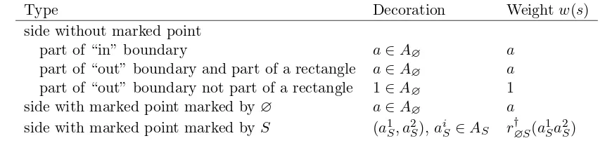
5.4.2 Examples: multiplication and comultiplication in the open sector
As an example we will consider the arc graphs given in Fig.5. This triangle gives a correlation function, which when dualized on the bottom edge yields a multiplication and when dualized on the top two edges yields a comultiplication. A more familiar form is given in the Sullivan case; see Section 6.5.1below.
Given
a=a(2)T ⊗a1⊗ · · · ⊗an⊗a(1)S ∈Bn(AT, A, AS)
and
a′ =a(2)S ⊗a′1⊗ · · · ⊗am′ ⊗a(1)U ∈Bm(AS, A, AU)
their product which lies in Bn+m+1(AT, A, AU) is given by
mT SU(aa′) =aT(2)⊗a1⊗ · · · ⊗an⊗r
†
S(a
(1)
S a
(2)
S )⊗a′1⊗ · · · ⊗a′m⊗a
(1)
U .
The calculation goes as follows. The integrals are R rT†(a(1)T aT(2)) = RT a(1)T a(2)T which dualizes to idT(a(1)T ) = a(1)T and likewise for U. For the rectangles we get either R aia′′j or
R
a′
ia′′k which
dualize to id(ai) and id(aj). Finally we get Rr†S(a(1)S a(2)S )a′′n+1 which dualizes to r†S◦µ.
The corresponding co-products by dualizing are ∆T SU : B(AT, A, AU) → B(AU, A, AS)⊗
B(AS, A, AT) let
Figure 5. To the left: an arc graph Γ in a triangle yielding the open sector multiplication or the co-multiplication. To the right: a discrete summand ofPΓ with weights 2 and 3 together with a decoration of it.
∆T SU(a′′) =
X
i
a(2)T ⊗a′′1⊗ · · · ⊗a′′i−1⊗(rS(ai))(1)⊗(rS(aj))(2)⊗ai+1⊗ · · · ⊗an⊗a(1)U ,
where ∆S(rS(ai) = (rS(ai))(1))⊗(rC(aj))(2)) using Sweedler’s notation. For this we dualize
R
rS†(a(1)S aS(2))a′′n+1=RS⊗S(a(1)S ⊗a(2)S ∆S(rS(a′′i)).
6
Open/closed string topology
6.1 Cell actions
We will now consider chain complexes whose chain groups are generated by generators indexed by arc graphs. The basic way to obtain actions of these chain complexes is to let each generator act via the graph that indexes it as we explain below.
Analogously to the purely closed situation [7, 8] there are two cases which we can study. The open/closed moduli space case and the open/closed Sullivan PROP case. Although their basic underpinnings are the same the details are slightly different, again as in [7, 8]. For the open/closed PROP case, we will have to change the actions of the weighted arc graphs slightly by using degeneracy maps. This is what corresponds to the breaking of the symmetry between “ins” and “outs” in the PROP itself. After putting in these degeneracies, we obtain a dg-PROP action on the cell level. We will give the full details below. The moduli space case is discussed further in Section 7.
6.2 The open/closed Sullivan c/o-colored topological quasi-PROP
So far we have only a partial gluing structure. At the expense of having associativity only up to homotopy, we can rectify this partial structure to a full open/closed colored structure (see the Ap-pendix for a definition). Again without being too technical this means that we will have PROP gluings for two given elements α ∈Sullgc/o(n1, n2, m1, m2) and α′ ∈Sullg
c/o
(n2, n3, m3, m4) and
a paring of the closed “out” windows ofαand the “in” windows ofα. Likewise given elements and appropriate pairings there are gluingsα∈Sullgc/o(n1, n2, m1, m2) andα′ ∈Sullg
c/o
(n3, n4, m2, m3)
on all the open windows. Or even gluing all “in” to all “out” windowsα∈Sullgc/o(n1, n2, m1, m2)
and α′∈Sullgc/o(n
2, n3, m2, m3).
Given two elements α ∈ Sullgc/o(n1, n2, m1, m2) and α′ ∈ Sullg c/o
(n3, n4, m2, m3), the flow
depends on the choice of a pairing of open “in” windows of α′ and “out” windows of α and scales the weights of all the arcs incident to the m2 open “in” windows of α′ simultaneously.
Given such a pairing the flow at timet scales each weight of an arc to an “in” windoww′ of α′ by the factor of 1−t(α(w)/α(w′)−1) wherewis the window ofαpaired withw. At time 1, each window has the weight of its partner under the paring. Now glue using the previously established gluings on all windows. Since the partial structure was bi-modular, it does not matter in which order the gluings are performed. We can repeat the analogous procedure for open windows or all windows at once. The proof that these gluings are associative up to homotopy, which is the definition of a topological quasi-PROP goes along the same line of arguments as in [7, Section 5.6]:
Proposition 6.1. The open/closed Sullivan spaces Sullgc/o(n1, n2, m1, m2) form a (two-colored) brane labelled topological quasi-PROP.
Proof . The two colors are open and closed. We can either choose to glue only these, or glue both open and closed windows at one. The brane labelling is just given by the left and right brane labels of each window. The associativity up to homotopy comes from the fact that we used a flow. Flowing backwards interpolates between the different bracketings. These flow of course is only on the non-deleted arcs, which are the same set in both bracketings. An arc is deleted if it passes through the preimage of the glued windows. This condition is the same for
both iterations in the associativity check.
Notice that we have rectified the partial structure on the topological level, but we had to pay the price of relaxing associativity. This weaker structure of course induces a strict structure on the homology.
Corollary 6.2. The homology open/closed Sullivan spaces Sullgc/o(n1, n2, m1, m2)form a ( two-colored) brane labelled PROP.
The surprising fact is that although there is only the weaker structure on the topological level, there is already a strict structure on the chain level, when using the correct chains. This is the underlying principle of our constructions.
6.3 A CW model for Sullc/o
This paragraph is an application of the methods set forth in [7]. We define the following subspaces of Sullgc/o(n1, n2, m1, m2) we let Sullc/o1(n1, n2, m1, m2) be the subspace of all α ∈
g
Sullc/o(n1, n2, m1, m2) such that theα weight of each “in” window is 1.
Proposition 6.3. Sullc/o
1(n1, n2, m1, m2) is a CW complex, is a sub-topological quasi-PROP and is a deformation retract of Sullgc/o(n1, n2, m1, m2). The dimension k cells of this complex are indexed by arc graphs of Sullivan type withk+ 1 arcs and their attaching maps are given by deleting arcs and identifying this boundary with the cell of lower dimension.
arc graph Γ of Sullivan type on a brane labelled windowed surface F, we obtain a cell C(Γ) whose interior ˙C(Γ) is given by a product of open simplices ˙∆k:
˙
C(Γ) = Y
w∈{“in” windows ofF} ˙
∆|{arcs incident tow}|.
The statement about the attaching maps follows directly from the topology in Sullgc/o, where we simply delete an arc in the limit where its weight goes to zero. The fact that this is a sub-topological quasi PROP is immediate upon noticing that the property that theαweight of each “in” window is one is stable under the operation of gluing.
Since the gluing a window withnarcs to a window withm arcs produced at mostn+m−1 arcs we see that the gluing maps are indeed cellular and there are induced maps on the cellular level.
It remains to prove that these maps are associative on the nose. This follows in the same way as in [7, Theorem 5.33]. The proof there essentially goes over to the current situation for the closed part. The open part is actually simpler, since we do not have to worry about the condition of “twisted at the boundary”, since we keep the punctures upon gluing.
Theorem 6.4. The cellular chains of Sullc1/o(n1,n2,m1,m2) are an open/closed colored brane labelled PROP cell model for the spaces Sullgc/o(n1, n2, m1, m2).
Proof . This follows directly from the proposition.
Corollary 6.5. There is a open/closed brane labelled PROP structure on the free Abelian group generated by arc graphs of Sullivan type induced by the corresponding structure on the cellular chains of Sullc1/o.
Proof . This is defined simply by the identification of the free Abelian groups of cellular chains which are generated by the C(Γ) and the free Abelian groups generated by the respective
graphs.
Notice that in this structure when gluing Γ and Γ′ we obtain all the graphs that can appear combinatorially by giving arbitrary weights in Γ and Γ′ matching on the windows that are glued, with the extra condition that the arcs of the glued graph have the maximal number, i.e. the corresponding cell has the maximum possible dimension.
6.4 The open/closed string topology action on brane labelled Hochschild complexes
6.4.1 The correlators in the Sullivan case
In the Sullivan graph case, when decorating and calculating the weights, we also distinguish between “in” and “out” boundaries. We will use the correlators Yi/o(Γ) which are obtained from the Y((Γ, w)) by using the degeneracies.
Given an discretely weighted arc family of Sullivan type (Γ, w) on a surfaceF with “in” and “out” boundary markings. Let
a=a(in)⊗a(out)∈ O
w∈“in” windows ofα
B(β(w))⊗ O
w∈“out” windows ofα
B(β(w)),
we definesa asa(in)⊗sa(out) where sa(out) is defined as follows:
Let a(out) = Naw. On the window w of the discrete family enumerate all components
starting at 0. Let n1 < n2. . . nk be the boundary pieces between non-parallel arcs, which are
not flags. Then we set
saw :=sn1sn2. . . snkaw.
Givena∈a(in)⊗a(out) we define
Yi/o(a) :=Y(sa).
According to this the correlators will again be multilinear maps
Yi/o(α) := O
w∈Windows of α
B(β(w))→k,
where these functions are homogeneous and their homogeneous components are zero by definition unless aw ∈Bα(w)−1−(β(w), A).
6.4.2 Decorations in the string topology case
The above procedure is tantamount to changing the decorations as follows:
Table 2. Weights for open/closed string topology.
Type Decoration Weight w(s)
side without marked point
part of “in” boundary a∈A∅ a
part of “out” boundary and part of a rectangle a∈A∅ a part of “out” boundary not part of a rectangle 1∈A∅ 1 side with marked point marked by∅ a∈A∅ a
side with marked point marked byS (a1S, a2S),aiS ∈AS r†∅S(a1Sa2S)
In [8] we used angle markings to this effect. In that language the table above is the analog of the decorations for the angle markings in the PROP case. The angles correspond exactly to the components of the boundary minus the arcs.
6.5 The action
Theorem 6.6. The open/closed β brane labelled open/closed dg-PROP cell model of Sullgc/o provided by Sullc1/o acts in a brane labelled open/closed dg-PROP fashion on the brane labelled Hochschild complexes for a β-Frobenius algebra which satisfies the Euler condition (E).
This has an immediate geometric consequence by using β Frobenius algebras coming form the geometric data of Section 4.1.5. Notice that in this case the bar complex B(∅,∅)) after
dualizing computes H∗(LM) whereLM is the free loop space [6] and the bar complex B(b, b′) after dualizing computes H∗(P M, Nb, Nb′) where P M(Nb, N
b′) is the space of paths which start
inNb and end in Nb′.
Corollary 6.7. If M is a simply connected compact manifold with a given set of D-branes realized by submanifolds Nb :b∈ B then there are open closed string topology type operations on
H∗(LM) and the various H∗(P M, Nb, Nb′).
Here define new operations through the E2 term of the respective spectral sequence. One
actually can do it for theE1term; confer [8]. This is what we call string topology type operations.
Figure 6. Gluing with angle labels in [8], in the current terminology the label 0 corresponds to a side without marked point on an “out” boundary that is not part of a rectangle.
Proof of Theorem 6.6. There are two things left to prove, the dg-properties and the compati-bility of the gluings on both sides of the action. We fist show the dg-properties. In the closed case the argument is the same as in [8, Section 4.2.1]. It basically relies on the fact that the co-multiplication and the multiplication are dual to each other. The argument carries over to the open case upon noticing that the only relevant case is the one where we locally consider an arc which has no parallel arc, as otherwise the terms of the differential cancel out. The only new case is when this arc is the only arc in the window. In this case (unlike in the closed case) removing the incident arc will still leave two decorations. In all other cases one of the decorations before removing the arc will be by 1. In this new case there are however two decorations before and after removing the arc due to the new rules of decorating on open windows, and hence the right hand side of the equations (4.7) and (4.8) of [8] still give the correlators on the surface with the arc removed.
The argument that the gluings on the Hochschild side in view of Theorem 5.1 and the geometric side coincide is completely analogous to [8, Theorem 4.4]. There are two steps in the argument. The first is that on the cellular chain side, only the graphs with maximal dimension appear and we have to check that only these appear on the Hochschild side. This is forced by the labelling. This labelling is equivalent to considering the gluing of [8] for angle labelled graphs (see Fig. 6). If does not want to take this detour one can prove this directly by noticing that the degeneracies duplicate edges on gluing. Now with this gluing the number of arcs is always maximal after gluing. On the Hochschild side, this is automatic as the number of “in” variables has to be equal to the number of “out” variables in order to obtain a non-zero gluing. The second step is to check that the actions given by the discretized arcs coincide before and after gluing. This is the content of Theorem5.1. The surprising new feature is that among the new local gluings coming from the open sector the compatibility holds only if additionally the
condition (E) is satisfied.
6.5.1 Examples multiplication and comultiplication
in the open sector in the string topology case
As an example we will consider the arc graphs given in Fig.5 but now with the Sullivan deco-ration. Given
a=a(2)T ⊗a1⊗ · · · ⊗an⊗a(1)S ∈Bn(AT, A, AS)
and
their product now lies inBn+m(AT, A, AU) and is given by
mT SU(aa′) =
Z
S
a(1)S a(2)S
a(2)T ⊗a1⊗ · · · ⊗an⊗a′1⊗ · · · ⊗a′m⊗a(1)U .
The calculation goes as follows. The integrals are R rT†(a(1)T aT(2)) = RTa(1)T a(2)T which dualizes to idT(a(1)T ) = a(1)T and likewise for U. For the rectangles we get either R aia′′j or
R
a′ia′′k which dualize to id(ai) and id(aj). Finally we getR rS†(aS(1)a(2)S )1 =RSa(1)S a(2)S which gives the factor
in front.
The corresponding co-products ∆T SU : B(AT, A, AU) → B(AU, A, AS)⊗B(AS, A, AT) are
left unchanged.
7
Moduli space actions
In the moduli spaces case, there an associated chain complex indexed by graphs. The difficulties in this case are manifold. First the cells of the chain complex are open cells. As we saw in [7, 8], the way to deal with this is to pass to the associated graded complex and look at the actions induced from the topological level there. Now there are new problems that arise in the open/closed case. While in the purely closed situation, the “forbidden” gluings which on the topological level gave rise to elements outside the moduli space were codimension one, here there are “forbidden” gluings for whole cells. An example is given in Figs. 7 and 8. We can deal with this by restricting the cells to come from an open/closed duality subspaces of moduli space. Also there are problems since we have to deal with internal marked points.
7.1 Point clusters
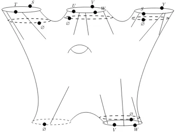
The property of moduli space that only once punctured polygons may appear among the com-plementary regions is very fragile under gluing. Not even the inclusion of the open and closed sectors into each other is stable with respect to this condition. So we will allow polygons with an arbitrary number of punctures. Using Strebel differentials, we can put a conformal structure on such a piece and have one distinguished point for this polygon. We now choose the geometric interpretation that all the points in the polygon with their brane labels are a cluster of points located at that distinguished point. We can think of these points as labelled “bosons” sitting on top of each other. In this sense they are equivalent to one internal marked point with a multiple brane label. This is very close to the moduli spaces considered in [13].
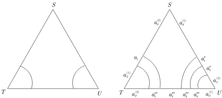
7.2 Open/closed duality
In [11] we saw that the open/closed duality holds on the chain level. This basically means that any element of Arc can be decomposed into a piece which is purely closed and cylinders whoseg one end is closed. This is simply obtained by cutting on a closed curve parallel to each boundary. If the boundary is already closed there is no need to cut. An example of this is given in Fig. 9. Notice the since we are cutting, we have the free choice of a point on the boundary and hence the pieces are not unique. They are of course unique up to twisting on the boundary, with the one parameter family on the annulus with closed windows, which is equivalent to moving a marked point marked by ∅ along the boundary. On the chain level this does however not hold for the
whole space and hence we will impose this condition.
Figure 7. A gluing of two elements of moduli space whose result does not lie in the moduli space. The window ABis glued to windowDE and the resulting element is not quasi-filling anymore.
A main result of [7] is that elements of open cells of two purely closed quasi-filling arc graphs are not in general position only in codimension one. This was enough to induce an operad structure on the associated graded of the chains.
Now, we also have problems with gluings of the type where two flags of a window belong to the same complementary region, e.g. the case e) 2) discussed in Section 5.3.3.
Definition 7.2. We say an open window of an arc familyα is degenerate if its flags are both part of the boundary of a complementary region, but are not an edge of this boundary. The latter can only happen if there is only one marked point on the boundary. This case will be non-degenerate.
Anarc family is non-degenerate if it has no degenerate windows.
7.2.1 Cell complexes
For aβ arc graphα on F, we let C(α) be the set of all projective weightings on α. Recall that a weighting is by positive reals, so that this set is just the open inside of a cell.
The space Arc(F, β)(n, m) :=Arc(g F, β)(n, m)/R>0 has decomposition into these open cells
Figure 8. Gluing of two cells of moduli space whose result does not lie in the moduli space. The gluing is along the windowsST which face each other. Again the result is not quasi-filling.
Figure 9. Open/closed duality: cut on the dotted lines.
This gives a complex whose generators are the open cells and whose boundary is given by the differential in the associated CW complex. The terms in the sum are only over those graphs which appear in the boundary. These are the subgraphs with one fewer edge.
1. The complementary regions are only polygons possibly with punctures of any finite num-ber.
2. The arc family admits a decomposition under the open/closed duality as above such that
(a) the pieces are in general position with respect to the boundaries obtained by cutting and
(b) the annuli appearing in the decomposition are non-degenerate.
In particular we let c/oMs,βg,δ1,...,δn be the component where the arc families are on (F
s g,n, β)
where the point clusters are given by the sets of marked points of cardinality si and s=Psi,
where a point cluster is the set of marked points within one polygonal complementary region.
Notice that the spacesc/oMs,βg,δ1,...,δn are stratified by the spaces
To avoid yet additional notation, we will think ofMs
g,δ1,...,δn and
c/oMs,β
g,δ1,...,δn as a subspace
of Arc(F, β)(n1, n2) where n1 is the number of δi = 1 andn1+n2 =nand F =Fg,ns .
The subspaces are then just given by the disjoint union of open cells of those graphs that satisfy the additional requirements.
There are gluings on the topological level, which are giving by scalings. Givenα and a win-dow w of it together with α′ and a window w′ on it, we scale all arcs α by α′(w′) and all arcs of α′ by α(w), just as in [12]. After the scaling the two windows have the same weight and we can glue. The structure we get is a two colored operad (open/closed) with the additional information of brane labels. We call such a structure a brane labelled open/closed operad.
Lemma 7.4. This gluing yields a brane-labelled open/closed operad structure. And this induces an operad structure on the complex of open cells.
Proof . On the topological level the only thing that is left to be checked is the associativity. Adapting [12] this is straightforward. For the chains, we notice that the set obtained from composing cells is a union of cells and proceed as in [7].
If we only stick to basic brane labels, we would need to introduce more colors, which would be as usual pairs (S, T) of S, T 6=∅or (∅,∅).
Lemma 7.5. The open cell complexes of Arc(F, β)(n1, n2) are graded by dimension – which for C˙(Γ)is the number of arcs minus one – and the induced operad structure respects the corre-sponding filtration and hence passes to the associated graded complexes.
Proof . This follows from the fact that when gluing two windows withkandlarcs, the maximal
number isk+l+ 1.
Proposition 7.6. The associated graded of the complexes of open cellsc/oMs,β
g,δ1,...,δn form a sub-operad of the associated graded of the complexes of open cells of Arc(F, β)(n1, n2).
To each such cell ˙C(Γ) we can associate the correlation functionY(Γ) acting on the approp-riate Hochschild co-chains or bar complexes. Now since we passed to the associated graded on the moduli space side, we will have to do the same thing on the algebraic side. This is accomplished by grading with respect to the number of comultiplications, analogous to [8] and then passing to the associated graded. The resulting objects can naturally be called aβ-labelled Hom operad.
Theorem 7.7. There is an operadic cell model associated to the β-brane labelled open/closed moduli spacesc/oMs,βg,δ1,...,δn which acts onβ-labelled Hochschild co-chains via operadic correlation functions with values in a β-labelled Hom operad.
Remark 7.8. On the image this operation is dg with respect to the induced differential.
8
Outlook
Again like in [9, 10] we can consider the stabilization. We see that in this case, we need that all the Frobenius algebras AS are (normalized) semi-simple in order to pass to the appropriate
stabilization.
One case where this would be true would be in Landau–Ginzburg models. We are currently working on the details of this theory.
One can furthermore ask about the modular operad structure on the moduli space. Then further technical complications arise from the intricate structure of the flows defining the chain level structure of the c/o structure in [11]. In this case we will show that there is an underlying solution to the quantum master equation.
A
Appendix: operadic, PROPic and c/o structures
A.1 The def inition of a c/o structure
Specify an object O(S, T) in some fixed symmetric monoidal category for each pairS andT of finite sets. A G-coloring on O(S, T) is the further specification of an objectGin this category and a morphism µ : S⊔T → Hom(O(S, T),G), and we shall let Oµ(S, T) denote this pair of
data.
A G-colored “closed/open” or c/o structure is a collection of such objects O(S, T) for each pair of finite sets S, T together with a choice of weighting µ for each object supporting the following four operations which are morphisms in the category:
Closed gluing: ∀s∈S,∀s′ ∈S′ withµ(s) =µ′(s′),
◦s,s′ : Oµ(S, T)⊗ O
µ′(S′, T′)→ O
µ′′(S⊔S′− {s, s′}, T ⊔T′); Closed self-gluing: ∀s, s′ ∈S with µ(s) =µ(s′) and s6=s′,
◦s,s′ : Oµ(S, T)→ Oµ′′(S− {s, s′}, T);
Open gluing: ∀t∈T,∀t′ ∈T′ withµ(t) =µ′(t′),
•t,t′ : Oµ(S, T)⊗ Oµ′(S′, T′)→ Oµ′′(S⊔S′, T⊔T′− {t, t′});
Open self-gluing: ∀t, t′ ∈T withµ(t) =µ(t′) andt6=t′,
![Figure 6. Gluing with angle labels in [8], in the current terminology the label 0 corresponds to a sidewithout marked point on an “out” boundary that is not part of a rectangle.](https://thumb-ap.123doks.com/thumbv2/123dok/912655.900483/24.612.136.491.54.203/figure-gluing-current-terminology-corresponds-sidewithout-boundary-rectangle.webp)