El e c t ro n ic
Jo ur
n a l o
f P
r o
b a b il i t y
Vol. 15 (2010), Paper no. 21, pages 654–683. Journal URL
http://www.math.washington.edu/~ejpecp/
On the critical point of the Random Walk Pinning Model in
dimension
d
=
3
∗
Quentin Berger
Laboratoire de Physique, ENS Lyon Université de Lyon
46 Allée d’Italie, 69364 Lyon, France e-mail: [email protected]
Fabio Lucio Toninelli
CNRS and Laboratoire de Physique, ENS Lyon Université de Lyon
46 Allée d’Italie, 69364 Lyon, France e-mail: [email protected]
Abstract
We consider the Random Walk Pinning Model studied in[3]and[2]: this is a random walkXon
Zd, whose law is modified by the exponential ofβ timesLN(X,Y), the collision local time up to
timeNwith the (quenched) trajectoryY of anotherd-dimensional random walk. Ifβexceeds a certain critical valueβc, the two walks stick together for typicalY realizations (localized phase). A natural question is whether the disorder is relevant or not, that is whether thequenched and annealed systems have the same critical behavior. Birkner and Sun[3]proved thatβc coincides with the critical point of theannealed Random Walk Pinning Model if the space dimension is d=1 ord=2, and that it differs from it in dimensiond≥4 (ford≥5, the result was proven also in[2]). Here, we consider the open case of themarginal dimensiond=3, and we prove non-coincidence of the critical points.
Key words:Pinning Models, Random Walk, Fractional Moment Method, Marginal Disorder. AMS 2000 Subject Classification:Primary 82B44, 60K35, 82B27, 60K37.
Submitted to EJP on December 15, 2009, final version accepted April 11, 2010.
1
Introduction
We consider the Random Walk Pinning Model (RWPM): the starting point is a zero-drift random walkX on Zd (d ≥1), whose law is modified by the presence of a second random walk, Y. The trajectory of Y is fixed (quenched disorder) and can be seen as the random medium. The modifi-cation of the law of X due to the presence of Y takes the Boltzmann-Gibbs form of the exponen-tial of a certain interaction parameter, β, times the collision local time of X andY up to time N,
LN(X,Y):=
P
1≤n≤N1{Xn=Yn}. Ifβ exceeds a certain threshold valueβc, then for almost every
real-ization ofY the walkX sticks together withY, in the thermodynamic limitN → ∞. If on the other handβ < βc, then LN(X,Y)iso(N)for typical trajectories.
Averaging with respect to Y the partition function, one obtains the partition function of the so-called annealed model, whose critical pointβcannis easily computed; a natural question is whether
βc 6= βcann or not. In the renormalization group language, this is related to the question whether
disorder isrelevantor not. In an early version of the paper[2], Birkneret al. proved thatβc6=βann c
in dimensiond≥5. Around the same time, Birkner and Sun[3]extended this result tod=4, and also proved that the two critical pointsdo coincidein dimensionsd=1 andd=2.
The dimensiond=3 is themarginal dimensionin the renormalization group sense, where not even heuristic arguments like the “Harris criterion” (at least its most naive version) can predict whether one has disorder relevance or irrelevance. Our main result here is that quenched and annealed critical points differ also ind=3.
For a discussion of the connection of the RWPM with the “parabolic Anderson model with a single catalyst”, and of the implications ofβc 6=βcann about the location of the weak-to-strong transition
for the directed polymer in random environment, we refer to[3, Sec. 1.2 and 1.4].
Our proof is based on the idea of bounding the fractional moments of the partition function, together with a suitable change of measure argument. This technique, originally introduced in[6; 9; 10]for the proof of disorder relevance for the random pinning model with tail exponentα≥1/2, has also proven to be quite powerful in other cases: in the proof of non-coincidence of critical points for the RWPM in dimension d ≥ 4 [3], in the proof that “disorder is always strong” for the directed polymer in random environment in dimension(1+2)[12]and finally in the proof that quenched and annealed large deviation functionals for random walks in random environments in two and three dimensions differ[15]. Let us mention that for the random pinning model there is another method, developed by Alexander and Zygouras [1], to prove disorder relevance: however, their method fails in the marginal situationα=1/2 (which corresponds tod=3 for the RWPM).
To guide the reader through the paper, let us point out immediately what are the novelties and the similarities of our proof with respect to the previous applications of the fractional moment/change of measure method:
• while the scheme of the proof of our Theorem 2.8 has many points in common with that of
[10, Th. 1.7], here we need new renewal-type estimates (e.g. Lemma 4.7) and a careful application of the Local Limit Theorem to prove that the average of the partition function under the modified measure is small (Lemmas 4.2 and 4.3).
2
Model and results
2.1
The random walk pinning model
Let X ={Xn}n≥0 andY ={Yn}n≥0 be two independent discrete-time random walks onZd, d ≥1,
starting from 0, and letPX andPY denote their respective laws. We make the following assumption:
Assumption 2.1. The random walkX is aperiodic. The increments(Xi−Xi−1)i≥1 are i.i.d.,
sym-metric and have a finite fourth moment (EXkX1k4<∞, wherek · kdenotes the Euclidean norm
onZd). Moreover, the covariance matrix ofX1, call itΣX, is non-singular.
The same assumptions hold for the increments ofY (in that case, we callΣY the covariance matrix ofY1).
For β ∈ R,N ∈ Nand for a fixed realization of Y we define a Gibbs transformation of the path
measurePX: this is the polymer path measurePβ
N,Y, absolutely continuous with respect toPX, given
by
dPβ
N,Y
dPX (X) =
eβLN(X,Y)1
{XN=YN}
ZNβ,Y
, (1)
where LN(X,Y) =
N
P
n=1 1{X
n=Yn}, and where
ZNβ,Y =EX[eβLN(X,Y)1
{XN=YN}] (2)
is the partition function that normalizesPβ
N,Y to a probability.
Thequenchedfree energy of the model is defined by
F(β):= lim
N→∞
1
N logZ
β
N,Y =N→∞lim
1
NE
Y[logZβ
N,Y] (3)
(the existence of the limit and the fact that it isPY-almost surely constant and non-negative is proven in[3]). We define also theannealedpartition functionEY[ZNβ,Y], and theannealedfree energy:
Fann(β):= lim
N→∞
1
N logE
Y[Zβ
N,Y]. (4)
We can compare thequenchedandannealedfree energies, via the Jensen inequality:
F(β) = lim
N→∞
1
NE
Y[logZβ
N,Y]6 Nlim→∞
1
NlogE
Y[Zβ
N,Y] =F
ann(β). (5)
The properties ofFann(·)are well known (see the Remark 2.3), and we have the existence of critical points[3], for bothquenchedandannealedmodels, thanks to the convexity and the monotonicity of
Definition 2.2(Critical points). There exist06βcann6βc depending on the laws of X and Y such
that: Fann(β) =0if β 6βcann and Fann(β)> 0ifβ > βcann; F(β) =0if β 6βc and F(β) >0if
β > βc.
The inequalityβcann6βc comes from the inequality (5).
Remark 2.3. As was remarked in[3], theannealedmodel is just the homogeneous pinning model
[8, Chapter 2]with partition function
EY[Zβ
N,Y] =EX−Y
exp β
N
X
n=1
1{(X−Y)n=0} !
1{(X−Y)N=0}
which describes the random walkX−Y which receives the rewardβ each time it hits 0. From the well-known results on the homogeneous pinning model one sees therefore that
• Ifd =1 or d =2, theannealedcritical pointβann
c is zero because the random walk X−Y is
recurrent.
• Ifd≥3, the walkX−Y is transient and as a consequence
βcann=−log1−PX−Y (X −Y)n6=0 for every n>0>0.
Remark 2.4. As in the pinning model[8], the critical pointβc marks the transition from a delocal-ized to a localdelocal-ized regime. We observe that thanks to the convexity of the free energy,
∂βF(β) = lim
N→∞
Eβ
N,Y
1
N
N
X
n=1
1{XN=YN}
, (6)
almost surely in Y, for every β such that F(·) is differentiable at β. This is the contact fraction betweenX andY. Whenβ < βc, we haveF(β) =0, and the limit density of contact betweenX and
Y is equal to 0: Eβ
N,Y
PN
n=11{XN=YN} = o(N), and we are in the delocalized regime. On the other
hand, ifβ > βc, we haveF(β)>0, and there is a positive density of contacts betweenX andY: we
are in the localized regime.
2.2
Review of the known results
The following is known about the question of the coincidence of quenched and annealed critical points:
Theorem 2.5. [3]Assume that X and Y are discrete time simple random walks onZd. If d=1or d=2, the quenched and annealed critical points coincide:βc=βcann=0.
If d≥4, the quenched and annealed critical points differ:βc> βcann>0.
Actually, the result that Birkner and Sun obtained in[3]is valid for slightly more general walks than simple symmetric random walks, as pointed out in the last Remark in [3, Sec.4.1]: for instance, they allow symmetric walksX andY with common jump kernel and finite variance, provided that
PX(X1=0)≥1/2.
Remark 2.6. The method and result of[3]in dimensions d =1, 2 can be easily extended beyond the simple random walk case (keeping zero mean and finite variance). On the other hand, in the case d ≥4 new ideas are needed to make the change-of-measure argument of [3]work for more general random walks.
Birkner and Sun gave also a similar result ifX andY are continuous-time symmetric simple random walks onZd, with jump rates 1 andρ≥0 respectively. With definitions of (quenched and annealed) free energy and critical points which are analogous to those of the discrete-time model, they proved:
Theorem 2.7. [3]In dimension d =1and d=2, one hasβc=βcann=0. In dimensions d≥4, one
has0< βcann< βc for eachρ >0. Moreover, for d =4and for eachδ >0, there exists aδ >0such
thatβc−βcann≥aδρ1+δ for allρ∈[0, 1]. For d≥5, there exists a>0such thatβc−βcann≥aρfor
allρ∈[0, 1].
Our main result completes this picture, resolving the open case of the critical dimensiond=3 (for simplicity, we deal only with the discrete-time model).
Theorem 2.8. Under the Assumption 2.1, for d=3, we haveβc> βcann.
We point out that the result holds also in the case whereX (orY) is a simple random walk, a case which a priori is excluded by the aperiodicity condition of Assumption 2.1; see the Remark 2.11.
Also, it is possible to modify our change-of-measure argument to prove the non-coincidence of quenched and annealed critical points in dimensiond=4 for the general walks of Assumption 2.1, thereby extending the result of[3]; see Section 4.4 for a hint at the necessary steps.
NoteAfter this work was completed, M. Birkner and R. Sun informed us that in[4]they indepen-dently proved Theorem 2.8 for the continuous-time model.
2.3
A renewal-type representation for
Z
Nβ,YFrom now on, we will assume thatd≥3.
As discussed in[3], there is a way to represent the partition function ZNβ,Y in terms of a renewal processτ; this rewriting makes the model look formally similar to the random pinning model[8].
In order to introduce the representation of[3], we need a few definitions.
Definition 2.9. We let
1. pXn(x) =PX(Xn= x)and pnX−Y(x) =PX−Y (X−Y)n=x;
2. Pbe the law of a recurrent renewal τ ={τ0,τ1, . . .} withτ0 =0, i.i.d. increments and
inter-arrival law given by
K(n):=P(τ1=n) =
pXn−Y(0)
GX−Y where G
X−Y :=X∞
n=1
pnX−Y(0) (7)
(note that GX−Y <∞in dimension d ≥3);
4. for n∈Nand x∈Zd,
w(z,n,x) =z p
X n(x)
pX−Y n (0)
; (8)
5. ZˇNz,Y := z′
1+z′Z
β
N,Y.
Then, via the binomial expansion ofeβLN(X,Y)= (1+z′)LN(X,Y)one gets[3]
ˇ
ZNz,Y =
N
X
m=1
X
τ0=0<τ1<...<τm=N
m
Y
i=1
K(τi−τi−1)w(z,τi−τi−1,Yτi−Yτi−1) (9)
= EW(z,τ∩ {0, . . . ,N},Y)1N∈τ
,
where we defined for any finite increasing sequences={s0,s1, . . . ,sl}
W(z,s,Y) =
EX Ql
n=1z1{Xsn=Ysn}
Xs
0=Ys0
EX−Y Ql
n=11{Xsn=Ysn}
Xs0=Ys0
=
l
Y
n=1
w(z,sn−sn−1,Ysn−Ysn
−1). (10)
We remark that, taking theEY−expectation of the weights, we get
EYw(z,τi−τi−1,Yτ
i −Yτi−1)
=z.
Again, we see that theannealedpartition function is the partition function of a homogeneous pinning model:
ˇ
ZNz,,annY =EY[ZˇNz,Y] =EzRN1
{N∈τ}
, (11)
where we definedRN :=|τ∩ {1, . . . ,N}|.
Since the renewalτis recurrent, theannealedcritical point iszcann=1.
In the following, we will often use the Local Limit Theorem for random walks, that one can find for instance in[5, Theorem 3](recall that we assumed that the increments of bothX andY have finite second moments and non-singular covariance matrix):
Proposition 2.10(Local Limit Theorem). Under the Assumption 2.1, we get
PX(Xn=x) = 1 (2πn)d/2(detΣ
X)1/2
exp
− 1
2nx·
Σ−X1x+o(n−d/2), (12)
where o(n−d/2)is uniform for x ∈Zd.
Moreover, there exists a constant c>0such that for all x∈Zd and n∈N
PX(Xn= x)6cn−d/2. (13)
(We use the notation x· y for the canonical scalar product inRd.)
In particular, from Proposition 2.10 and the definition of K(·) in (7), we get K(n) ∼ cKn−d/2 as
n→ ∞, for some positivecK. As a consequence, ford=3 we get from[7, Th. B]that
P(n∈τ)n→∞∼ 1
2πcKpn
. (14)
Remark 2.11. In Proposition 2.10, we supposed that the walkX is aperiodic, which is not the case for the simple random walk. IfXis the symmetric simple random walk onZd, then[13, Prop. 1.2.5]
PX(Xn=x) =1{n↔x} 2
(2πn)d/2(detΣ
X)1/2
exp
− 1
2nx·
Σ−X1x+o(n−d/2), (15)
where+o(n−d/2)is uniform for x∈Zd, and wheren↔x means thatnandx have the same parity
(so thatx is a possible value forXn). Of course, in this caseΣX is just 1/dtimes the identity matrix. The statement (13) also holds.
Via this remark, one can adapt all the computations of the following sections, which are based on Proposition 2.10, to the case whereX (orY) is a simple random walk. For simplicity of exposition, we give the proof of Theorem 2.8 only in the aperiodic case.
3
Main result: the dimension
d
=
3
With the definition ˇF(z):= limN→∞ 1
Nlog ˇZ z
N,Y, to prove Theorem 2.8 it is sufficient to show that
ˇ
F(z) =0 for somez>1.
3.1
The coarse-graining procedure and the fractional moment method
We consider without loss of generality a system of size proportional toL= z1
−1 (the coarse-graining
length), that isN=mL, withm∈N. Then, forI ⊂ {1, . . . ,m}, we define
ZzI,Y :=EW(z,τ∩ {0, . . . ,N},Y)1N∈τ1E
I(τ)
, (16)
where EI is the event that the renewalτintersects the blocks (Bi)i∈I and only these blocks over
{1, . . . ,N}, Bi being theithblock of sizeL:
Bi:={(i−1)L+1, . . . ,i L}. (17)
Since the eventsEI are disjoint, we can write
ˇ
ZNz,Y := X
I ⊂{1,...,m}
ZzI,Y. (18)
Note that ZzI,Y = 0 if m ∈ I/ . We can therefore assume m∈ I. If we denote I = {i1,i2, . . . ,il}
ZzI,Y := X
a1,b1∈Bi1
a16b1
X
a2,b2∈Bi2
a26b2
. . . X
al∈Bil
K(a1)w(z,a1,Ya1)Z
z
a1,b1 (19)
. . .K(al−bl−1)w(z,al−bl−1,Yal −Ybl−1)Z
z al,N,
where
Zzj,k:=EW(z,τ∩ {j, . . . ,k},Y)1k∈τ
j∈τ (20)
is the partition function between j andk.
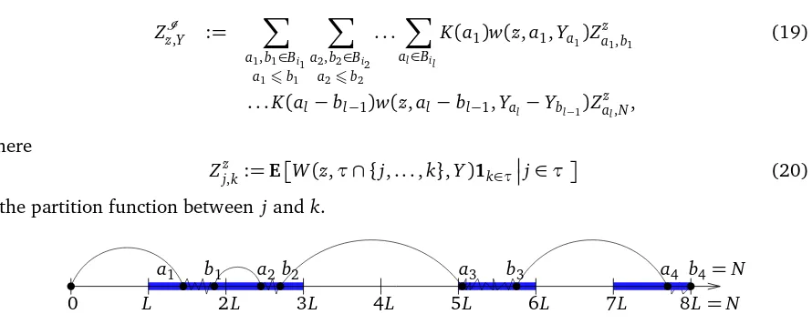
0 L 2L 3L 4L 5L 6L 7L 8L=N
[image:8.612.81.526.105.283.2]a1 b1 a2b2 a3 b3 a4 b4=N
Figure 1: The coarse-graining procedure. Here N = 8L (the system is cut into 8 blocks), and
I ={2, 3, 6, 8} (the gray zones) are the blocks where the contacts occur, and where the change of measure procedure of the Section 3.2 acts.
Moreover, thanks to the Local Limit Theorem (Proposition 2.10), one can note that there exists a constantc>0 independent of the realization ofY such that, if one takesz62 (we will takezclose to 1 anyway), one has
w(z,τi−τi−1,Yτi−Yτi−1) =z pτX
i−τi−1(Yτi−Yτi−1) pXτ−Y
i−τi−1(0)
≤c.
So, the decomposition (19) gives
ZzI,Y 6c|I | X
a1,b1∈Bi1
a16b1
X
a2,b2∈Bi2
a26b2
. . . X
al∈Bil
K(a1)Zaz
1,b1K(a2−b1)Z
z
a2,b2. . .K(al−bl−1)Z
z
al,N. (21)
We now eliminate the dependence onz in the inequality (21). This is possible thanks to the choice
L= 1
z−1. As each Z
z
ai,bi is the partition function of a system of size smaller than L, we getW(z,τ∩
{ai, . . . ,bi},Y) 6zLW(z = 1,τ∩ {ai, . . . ,bi},Y) (recall the definition (10)). But with the choice
L= 1
z−1, the factorz
Lis bounded by a constantc, and thanks to the equation (20), we finally get
Zaz
i,bi 6c Z
z=1
ai,bi. (22)
Notational warning: in the following, c,c′, etc. will denote positive constants, whose value may change from line to line.
We note Zai,bi := Zaz=1
i,bi and W(τ,Y) := W(z = 1,τ,Y). Plugging this in the inequality (21), we
finally get
ZzI,Y 6c′|I | X
a1,b1∈Bi1
a16b1
X
a2,b2∈Bi2
a26b2
. . . X
al∈Bil
where there is no dependence onzanymore.
The fractional moment method starts from the observation that for anyγ6=0
ˇ
F(z) = lim
N→∞
1
γNE
Y logZˇz N,Y
γ
6 lim inf
N→∞
1
NγlogE
YZˇz N,Y
γ
. (24)
Let us fix a value ofγ∈(0, 1) (as in[10], we will chooseγ= 6/7, but we will keep writing it as
γto simplify the reading). Using the inequality Panγ 6 Paγn (which is valid for ai ≥0), and combining with the decomposition (18), we get
EY
ˇ
ZNz,Yγ
6 X
I ⊂{1,...,m}
EY
ZzI,Yγ
. (25)
Thanks to (24) we only have to prove that, for somez>1, lim supN→∞EY
ˇ
ZNz,Yγ
<∞. We deal with the termEY
h
(ZzI,Y)γivia a change of measure procedure.
3.2
The change of measure procedure
The idea is to change the measurePY on each block whose index belongs toI, keeping each block independent of the others. We replace, for fixedI, the measurePY(dY)withgI(Y)PY(dY), where the function gI(Y) will have the effect of creating long range positive correlations between the increments ofY, inside each block separately. Then, thanks to the Hölder inequality, we can write
EY
ZzI,Yγ
=EY g
I(Y)γ
gI(Y)γ
ZzI,Yγ
6 EY h
gI(Y)−
γ
1−γ
i1−γ
EY h
gI(Y)ZzI,Yiγ. (26)
In the following, we will denote∆i =Yi−Yi−1 theithincrement of Y. Let us introduce, for K>0
andǫK to be chosen, the following “change of measure”:
gI(Y) =Y
k∈I
(1F
k(Y)6K+ǫK1Fk(Y)>K)≡ Y
k∈I
gk(Y), (27)
where
Fk(Y) =− X
i,j∈Bk
Mi j∆i·∆j, (28)
and
Mi j= p 1
LlogL
1
Æ
|j−i| if i6= j
Mii=0.
(29)
Let us note that from the form of M, we get that kMk2 := Pi,j∈B
1M
2
i j 6 C, where the constant
Let us deal with the first factor of (26):
EY h
gI(Y)−
γ
1−γ
i
=Y
k∈I
EY h
gk(Y)−
γ
1−γ
i =
PY(F1(Y)6K) +ǫ−
γ
1−γ
K P
Y(F
1(Y)>K)
|I |
. (30)
We now choose
ǫK :=PY(F1(Y)>K)
1−γ
γ (31)
such that the first factor in (26) is bounded by 2(1−γ)|I |62|I |. The inequality (26) finally gives
EY
ZzI,Y γ
62|I |EY h
gI(Y)ZzI,Y iγ
. (32)
The idea is that whenF1(Y) is large, the weight g1(Y) in the change of measure is small. That is
why the following lemma is useful:
Lemma 3.1. We have
lim
K→∞lim supL→∞
ǫK = lim
K→∞lim supL→∞
PY(F1(Y)>K) =0 (33)
Proof. We already know thatEY[F1(Y)] =0, so thanks to the standard Chebyshev inequality, we
only have to prove thatEY[F1(Y)2]is bounded uniformly inL. We get
EY[F1(Y)2] = X
i,j∈B1
k,l∈B1
Mi jMklEY(∆i·∆j)(∆k·∆l)
= X
{i,j}
Mi j2EY(∆i·∆j)2 (34)
where we used thatEY(∆i·∆j)(∆k·∆l)= 0 if {i,j} 6= {k,l}. Then, we can use the
Cauchy-Schwarz inequality to get
EY[F1(Y)2]6
X
{i,j}
Mi j2EYh∆i2∆j2i 6kMk2σ4Y :=kMk2EY(||Y1||2)
2
. (35)
We are left with the estimation ofEY h
gI(Y)ZzI,Yi. We setPI :=P EI,N∈τ, that is the prob-ability forτ to visit the blocks (Bi)i∈I and only these ones, and to visit also N. We now use the following two statements.
Proposition 3.2. For anyη >0, there exists z > 1sufficiently close to1(or L sufficiently big, since L= (z−1)−1) such that for everyI ⊂ {1, . . . ,m}with m∈ I, we have
EY h
gI(Y)ZzI,Yi 6η|I |PI. (36)
Lemma 3.3. [10, Lemma 2.4] There exist three constants C1 = C1(L), C2 and L0 such that (with i0:=0)
PI 6C1C2|I |
|I |
Y
j=1
1
(ij−ij−1)7/5 (37)
for L≥ L0and for everyI ∈ {1, . . . ,m}.
Thanks to these two statements and combining with the inequalities (25) and (32), we get
EY
ˇ
ZNz,Yγ
6 X
I ⊂{1,...,m}
EY
ZzI,Yγ
6C1γ X
I ⊂{1,...,m} |I |
Y
j=1
(3C2η)γ
(ij−ij−1)7γ/5. (38)
Since 7γ/5=6/5>1, we can set
e
K(n) = 1 e
cn6/5, where ec=
+∞
X
i=1
i−6/5<+∞, (39)
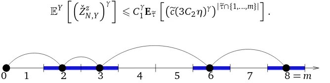
and Ke(·) is the inter-arrival probability of some recurrent renewal τe. We can therefore interpret the right-hand side of (38) as a partition function of a homogeneous pinning model of sizem(see Figure 2), with the underlying renewalτe, and with pinning parameter log[ec(3C2η)γ]:
EY
ˇ
ZNz,Yγ
6C1γEτe
h
ec(3C2η)γ|τe∩{1,...,m}|i. (40)
[image:11.612.135.469.377.461.2]0 1 2 3 4 5 6 7 8=m
Figure 2: The underlying renewalτeis a subset of the set of blocks(Bi)16i6m (i.e the blocks are
reinterpreted as points) and the inter-arrival distribution isKe(n) =1/ecn6/5.
Thanks to Proposition 3.2, we can takeηarbitrary small. Let us fixη:=1/((4C2)ec1/γ). Then,
EY
ˇ
ZNz,Y γ
6C1γ (41)
for everyN. This implies, thanks to (24), that ˇF(z) =0, and we are done.
Remark 3.4. The coarse-graining procedure reduced the proof of delocalization to the proof of Proposition 3.2. Thanks to the inequality (23), one has to estimate the expectation, with respect to the gI(Y)−modified measure, of the partition functions Zai,bi in each visited block. We will show
(this is Lemma 4.1) that the expectation with respect to this modified measure ofZai,bi/P(bi−ai ∈τ)
4
Proof of the Proposition 3.2
As pointed out in Remark 3.4, Proposition 3.2 relies on the following key lemma:
Lemma 4.1. For everyǫandδ >0, there exists L>0such that
EYg1(Y)Za,b6δP(b−a∈τ) (42)
for every a6b in B1such that b−a≥ǫL.
Given this lemma, the proof of Proposition 3.2 is very similar to the proof of[10, Proposition 2.3], so we will sketch only a few steps. The inequality (23) gives us
EY h
gI(Y)ZzI,Y i
6 c|I | X
a1,b1∈Bi1
a16b1
X
a2,b2∈Bi2
a26b2
. . . X
al∈Bil
K(a1)EY
gi1(Y)Za1,b1
K(a2−b1)EY
gi2(Y)Za2,b2
. . .
. . .K(al−bl−1)EY gi
l(Y)Zal,N
= c|I | X
a1,b1∈Bi1
a16b1
X
a2,b2∈Bi2
a26b2
. . . X
al∈Bil
K(a1)EYg1(Y)Za1−L(i1−1),b1−L(i1−1)
K(a2−b1). . . (43)
. . .K(al−bl−1)EY
g1(Y)Zal−L(m−1),N−L(m−1)
.
The terms with bi−ai ≥ ǫL are dealt with via Lemma 4.1, while for the remaining ones we just
observe thatEY[g1(Y)Za,b]≤P(b−a∈τ)since g1(Y)≤1. One has then
EY h
gI(Y)ZzI,Yi 6 c|I | X
a1,b1∈Bi1
a16b1
X
a2,b2∈Bi2
a26b2
. . . X
al∈Bil
K(a1)δ+1{b
1−a16ǫL}
P(b1−a1∈τ)
. . .K(al−bl−1)
δ+1{N−al6ǫL}
P(N−al∈τ). (44)
From this point on, the proof of Theorem 3.2 is identical to the proof of Proposition 2.3 in[10](one needs of course to chooseǫ=ǫ(η)andδ=δ(η)sufficiently small).
4.1
Proof of Lemma 4.1
Let us fixa,binB1, such thatb−a≥ǫL. The small constantsδandǫare also fixed. We recall that for a fixed configuration ofτ such that a,b ∈τ, we have EYW(τ∩ {a, . . . ,b},Y) = 1 because
z=1. We can therefore introduce the probability measure (always for fixedτ)
dPτ(Y) =W(τ∩ {a, . . . ,b},Y)dPY(Y) (45)
where we do not indicate the dependence ona andb. Let us note for later convenience that, in the particular casea=0, the definition (10) ofW implies that for any function f(Y)
Eτ[f(Y)] =EXEYf(Y)|Xi=Yi∀i∈τ∩ {1, . . . ,b}
With the definition (20) ofZa,b:=Zaz,=b1, we get
EYg1(Y)Za,b
=EYEg1(Y)W(τ∩ {a, . . . ,b},Y)1b∈τ|a∈τ
=bEEτ[g1(Y)]P(b−a∈τ), (47)
wherebP(·):=P(·|a,b∈τ), and therefore we have to show thatbEEτ[g1(Y)]6δ.
With the definition (27) of g1(Y), we get that for anyK
b
EEτ[g1(Y)]6ǫK+bEPτ F1<K
. (48)
If we chooseKbig enough,ǫK is smaller thanδ/3 thanks to the Lemma 3.1. We now use two lemmas
to deal with the second term. The idea is to first prove thatEτ[F1]is big with abP−probability close to 1, and then that its variance is not too large.
Lemma 4.2. For every ζ > 0 and ǫ > 0, one can find two constants u = u(ǫ,ζ) > 0 and L0 =
L0(ǫ,ζ)>0, such that for every a,b∈B1such that b−a≥ǫL,
b
PEτ[F1]≤uplogL≤ζ, (49)
for every L≥L0.
Chooseζ=δ/3 and fixu>0 such that (49) holds for every Lsufficiently large. If 2K =uplogL
(and therefore we can makeǫK small enough by choosing Llarge), we get that
b
EPτ F1<K 6 bEPτF1−Eτ[F1]6 −K
+Pb Eτ[F1]62K
(50)
6 1
K2bEEτ
F1−Eτ[F1]
2
+δ/3. (51)
Putting this together with (48) and with our choice ofK, we have
b
EEτ[g1(Y)]62δ/3+ 4 u2logLEbEτ
F1−Eτ[F1]2 (52)
forL≥L0. Then we just have to prove thatEbEτ
F1−Eτ[F1]
2
=o(logL). Indeed,
Lemma 4.3. For everyǫ >0there exists some constant c=c(ǫ)>0such that
b
EEτ F1−Eτ[F1]2 6c logL3/4 (53)
for every L>1and a,b∈B1 such that b−a≥ǫL.
We finally get that
b
EEτ[g1(Y)]62δ/3+c(logL)−1/4, (54)
and there exists a constantL1>0 such that forL>L1
b
4.2
Proof of Lemma 4.2
Up to now, the proof of Theorem 2.8 is quite similar to the proof of the main result in[10]. Starting from the present section, instead, new ideas and technical results are needed.
Let us fix a realization of τsuch that a,b∈τ(so that it has a non-zero probability underbP) and let us note τ∩ {a, . . .b} = {τRa = a,τRa+1, . . . ,τRb = b} (recall that Rn = |τ∩ {1, . . . ,n}|). We
observe (just go back to the definition of Pτ) that, if f is a function of the increments of Y in
{τn−1+1, . . . ,τn}, gof the increments in {τm−1+1, . . . ,τm}withRa <n6= m≤Rb, and ifhis a
function of the increments ofY not in{a+1, . . . ,b}then
Eτf {∆i}i∈{τ
n−1+1,...,τn}
g {∆i}i∈{τ
m−1+1,...,τm}
h {∆i}i∈{a/ +1,...,b} (56)
= Eτf {∆i}i∈{τ
n−1+1,...,τn}
Eτg {∆i}i∈{τ
m−1+1,...,τm}
EYh {∆i}i∈{/ a+1,...,b},
and that
Eτf {∆i}i∈{τ
n−1+1,...,τn}
=EXEYf {∆i}i∈{τ
n−1+1,...,τn}
|Xτ
n−1=Yτn−1,Xτn=Yτn
=EXEYf {∆i−τ
n−1}i∈{τn−1+1,...,τn}
|Xτn−τn−1=Yτn−τn−1
. (57)
We want to estimateEτ[F1]: since the increments∆i fori∈B1\{a+1, . . . ,b}are i.i.d. and centered
(like underPY), we have
Eτ[F1]:=
b
X
i,j=a+1
Mi jEτ[−∆i·∆j]. (58)
Via a time translation, one can always assume thata=0 and we do so from now on.
The key point is the following
Lemma 4.4. 1. If there exists1≤n≤Rb such that i,j∈ {τn−1+1, . . . ,τn}, then
Eτ[−∆i·∆j] =A(r)r→∞∼ CX,Y
r (59)
where r =τn−τn−1 (in particular, note that the expectation depends only on r) and CX,Y is a
positive constant which depends onPX,PY; 2. otherwise,Eτ[−∆i·∆j] =0.
Proof of Lemma 4.4Case (2). Assume thatτn−1<i≤τn andτm−1< j≤τm withn6=m. Thanks
to (56)-(57) we have that
Eτ[∆i·∆j] =EXEY[∆i|Xτ
n−1=Yτn−1,Xτn=Yτn]·E
XEY[∆
j|Xτm−1=Yτm−1,Xτm=Yτm] (60)
and both factors are immediately seen to be zero, since the laws of X and Y are assumed to be symmetric.
Case (1).Without loss of generality, assume thatn=1, so we only have to compute
wherer =τ1. Let us fixx ∈Z3, and denoteEYr,x[·] =E Y[
·Yr=x].
EY[∆i·∆jYr=x] = EY
r,x
h ∆i·EY
r,x
∆j∆ii
= EY
r,x
∆i· x−∆i r−1
= x
r−1·E
Y r,x
∆i− 1 r−1E
Y r,x
h ∆i2i
= 1
r−1
kxk2 r −E
Y r,x
h ∆12
i
,
where we used the fact that underPY
r,x the law of the increments{∆i}i≤ris exchangeable. Then, we
get
Eτ[∆i·∆j] =EXEY∆i·∆j1{Y
r=Xr}
PX−Y(Yr=Xr)−1 = EX
h
EY∆i·∆jYr=Xr
PY(Yr=Xr)
i
PX−Y(Yr=Xr)−1
= 1
r−1
EX
Xr2
r P
Y(Y r=Xr)
PX−Y(Yr=Xr)−1
−EXEYh∆121{Y r=Xr}
i
PX−Y(Yr=Xr)−1
= 1
r−1
EX
Xr
2
r P
Y(Y r=Xr)
PX−Y(Yr=Xr)−1−EXEYh∆12Yr=Xri .
Next, we study the asymptotic behavior of A(r) and we prove (59) with CX,Y = t r(ΣY) − t r(Σ−X1+ ΣY−1)−1. Note thatt r(Σ
Y) =EY(||Y1||2) =σ2Y. The fact thatCX,Y >0 is just a
conse-quence of the fact that, ifAand Bare two positive-definite matrices, one has thatA−B is positive definite if and only ifB−1−A−1 is[11, Cor. 7.7.4(a)].
To prove (59), it is enough to show that
EXEYh∆12Yr=Xr
ir→∞
→ EXEYh∆12 i
=σ2Y, (62)
and that
B(r):= EX
kXrk
2
r P Y(Y
r=Xr)
PX−Y(Xr=Yr)
r→∞
→ t r(Σ−X1+ ΣY−1)−1. (63)
To prove (62), write
EXEYh∆12Yr=Xri = EYh∆12PX(Xr=Yr)iPX−Y(Xr=Yr)−1
= X
y,z∈Zd
kyk2PY(Y1= y)
PY(Yr−1=z)PX(Xr= y+z)
PX−Y(Xr−Yr=0) . (64)
We know from the Local Limit Theorem (Proposition 2.10) that the term PX(Xr=y+z)
PX−Y(Xr−Yr=0) is uniformly
bounded from above, and so there exists a constantc>0 such that for all y ∈Zd X PY(Yr−1=z)PX(Xr= y+z)
If we can show that for every y fixed Zd the left-hand side of (65) goes to 1 as r goes to infinity, then from (64) and a dominated convergence argument we get that
EXEYh∆12Yr=Xr
ir→∞
−→ X
y∈Zd
kyk2PY(Y1= y) =σ2Y. (66)
We use the Local Limit Theorem to get
X
z∈Zd
PY(Yr−1=z)PX(Xr= y+z) =
X
z∈Zd cXcY
rd e
−2(r1−1)z·(Σ−
1
Y z)e−21r(y+z)·(ΣX−1(y+z)) +o(r−d/2)
= (1+o(1))X
z∈Zd cXcY
rd e
−21rz·(Σ−1
Y z)e−
1 2rz·(Σ−
1
X z) +o(r−d/2) (67)
where cX = (2π)−d/2(detΣX)−1/2 and similarly for cY (the constants are different in the case of simple random walks: see Remark 2.11), and where we used that y is fixed to neglect y/pr. Using the same reasoning, we also have (with the same constantscX andcY)
PX−Y(Xr=Yr) = X
z∈Zd
PY(Yr=z)PX(Xr=z)
= X
z∈Zd cXcY
rd e
−21rz·(Σ−1
Y z)e−
1 2rz·(Σ−
1
X z) +o(r−d/2). (68)
Putting this together with (67) (and considering that PX−Y(Xr = Yr) ∼ cX,Yr−d/2), we have, for every y ∈Zd
X
z∈Zd
PY(Yr−1=z)PX(Xr= y+z)
PX−Y(Xr−Yr=0)
r→∞
−→1. (69)
To deal with the termB(r)in (63), we apply the Local Limit Theorem as in (68) to get
EX Xr
2
r P
Y(Y r=Xr)
= cYcX rd
X
z∈Zd
kzk2
r e
−21rz·(Σ−
1
Y z)e−
1 2rz·(Σ−
1
X z) +o(r−d/2). (70)
Together with (68), we finally get
B(r) =
cYcX
rd P
z∈Zd k
zk2 r e
−21rz·((Σ−1Y +Σ−1X )z) +o(r−d/2)
cYcX
rd P
z∈Zde−
1 2rz·((Σ−
1
Y +Σ−
1
X )z) +o(r−d/2)
= (1+o(1))EkN k2, (71)
where N ∼ N 0,(Σ−Y1+ Σ−X1)−1 is a centered Gaussian vector of covariance matrix
(Σ−Y1+ Σ−X1)−1. Therefore,EkN k2=t r(Σ−Y1+ Σ−X1)−1and (63) is proven.
Remark 4.5. For later purposes, we remark that with the same method one can prove that, for any given k0 ≥ 0 and polynomials U and V of order four (so that EY[|U{∆k}k6k
0
|] < ∞and
EX[V(||Xr||/pr)]<∞), we have
EXEY
U{∆k
}k6k
0
V
Xr
p
r !
Yr=Xr
r→∞→ EYU{k∆kk}k6k
0
whereN is as in (71).
Let us quickly sketch the proof: as in (64), we can write
EXEY
U{k∆kk}k6k
0
V
kXrk
p
r
Yr=Xr
= (73)
X
y1,...,yk0∈Zd
U{kykk}k6k0
X
z∈Zd V
kzk
p
r
PX(Xr=z)
PY(Yr−k0=z−y1−. . .− yk0) PX−Y(Xr−Yr=0)
×PY(∆i= yi,i≤k0).
Using the Local Limit Theorem the same way as in (68) and (71), one can show that for any
y1, . . . ,yk 0
X
z∈Zd V
kzk p
r
PX(Xr=z)
PY(Yr−k
0=z−y1−. . .− yk0) PX−Y(Xr−Yr=0)
r→∞
→ EV(kN k). (74)
The proof of (72) is concluded via a domination argument (as for (62)), which is provided by uniform bounds onPY(Yr−k0=z−y1−. . .−yk0) andP
X−Y(X
r−Yr =0)and by the fact that the
increments ofX andY have finite fourth moments.
Given Lemma 4.4, we can resume the proof of Lemma 4.2, and lower bound the averageEτ[F1].
Recalling (58) and the fact that we reduced to the casea=0, we get
Eτ[F1] =
Rb X
n=1
X
τn−1<i,j≤τn Mi j
A(∆τn), (75)
where∆τn:=τn−τn−1. Using the definition (29) of M, we see that there exists a constantc>0
such that for 1<m≤L
m
X
i,j=1
Mi j≥ p c LlogL
m3/2. (76)
On the other hand, thanks to Lemma 4.4, there exists some r0>0 and two constants candc′such
thatA(r)≥ cr forr≥r0, andA(r)≥ −c′for everyr. Plugging this into (75), one gets
p
LlogLEτ[F1]≥c
Rb X
n=1
p
∆τn1{∆τn≥r0}−c
′ Rb X
n=1
(∆τn)3/21{∆τn6r0}≥c
Rb X
n=1
p
∆τn−c′Rb. (77)
Therefore, we get for any positiveB>0 (independent of L)
b
PEτ[F1]6gplogL 6bP
p 1
LlogL c
Rb X
n=1
p
∆τn−c′Rb
!
6uplogL
6 bP
p 1
LlogL c
Rb X
n=1
p
∆τn−c′
p
LB !
6uplogL
+bPRb>BpL
6 bP
Rb/2
Xp
∆τn≤(1+o(1))
u c
p
LlogL
+bP(Rb>B
p
Now we show that forB large enough, andL≥L0(B),
b
P(Rb>B
p
L)6ζ/2, (79)
whereζis the constant which appears in the statement of Lemma 4.2. We start with getting rid of the conditioning inbP(recall bP(·) = P(·|b∈τ)since we reduced to the case a=0). IfRb> B
p
L, then either |τ∩ {1, . . . ,b/2}| or |τ∩ {b/2+1, . . . ,b}| exceeds B2pL. Since both random variables have the same law underbP, we have
b
P(Rb>BpL)62bP
Rb/2>
B
2
p
L
≤2cP
Rb/2>
B 2 p L , (80)
where in the second inequality we applied Lemma A.1. Now, we can use the Lemma A.3 in the Appendix, to get that (recall b≤L)
P
Rb/2>
B 2 p L ≤P RL/2>
B 2 p L L→∞ → P |Z | p
2π ≥B cK
p
2
, (81)
withZ a standard Gaussian random variable andcK the constant such that K(n)∼ cKn−3/2. The inequality (79) then follows forB sufficiently large, andL≥ L0(B).
We are left to prove that forLlarge enough andusmall enough
b
P
Rb/2
X
n=1
p ∆τn6
u c
p
LlogL
6ζ/2. (82)
The conditioning inbPcan be eliminated again via Lemma A.1. Next, one notes that for any given
A>0 (independent ofL)
P
Rb/2
X
n=1
p ∆τn6
u c
p
LlogL 6P
ApL
X
n=1
p ∆τn6
u c
p
LlogL
+PRb/2<A
p
L. (83)
Thanks to the Lemma A.3 in Appendix and tob≥ǫL, we have
lim sup L→∞ P R b/2 p
L <A
≤P p|Z |
2π <AcK
r
2
ǫ
!
,
which can be arbitrarily small ifA=A(ǫ)is small enough, for Llarge. We now deal with the other term in (83), using the exponential Bienaymé-Chebyshev inequality (and the fact that the∆τn are
i.i.d.):
P
p 1
LlogL
AXpL
n=1
p ∆τn<
u c p logL
6e(u/c)plogLE
exp − r τ1
LlogL ApL
. (84)
To estimate this expression, we remark that, for Llarge enough,
E
1−exp
−
r
τ1
LlogL
=
∞
X
n=1
K(n)
1−e−
Æ n
LlogL
≥ c′
∞
X
n=1
1−e−
Æ n
LlogL
n3/2 ≥c
′′
r
logL
where the last inequality follows from keeping only the terms with n≤ L in the sum, and noting that in this range 1−e−
Æ n
LlogL ≥cpn/(LlogL). Therefore,
E
exp
−
r
τ1
LlogL ApL
6 1−c′′ r
logL L
!ApL
≤e−c′′AplogL, (86)
and, plugging this bound in the inequality (84), we get
P
p 1
LlogL
AXpL
n=1
p ∆τn6
u c
p
logL
6e[(u/c)−c′′A]plogL, (87)
that goes to 0 ifL→ ∞, provided thatuis small enough. This concludes the proof of Lemma 4.2.
4.3
Proof of Lemma 4.3
We can write
−F1+Eτ[F1] =S1+S2:=
b
X
i6=j=a+1
Mi jDi j+ ′
X
i6=j
Mi jDi j (88)
where we denoted
Di j = ∆i·∆j−Eτ[∆i·∆j] (89)
and
′
P
stands for the sum over all 1≤ i6= j ≤ L such that either i or j (or both) do not fall into
{a+1, . . . ,b}. This way, we have to estimate
Eτ[(F1−Eτ[F1])2]≤2Eτ[S12] +2Eτ[S22] (90)
= 2
b
X
i6=j=a+1
b
X
k6=l=a+1
Mi jMklEτ[Di jDkl] +2
′
X
i6=j ′
X
k6=l
Mi jMklEτ[Di jDkl].
Remark 4.6. We easily deal with the part of the sum where{i,j}={k,l}. In fact, we trivially bound
Eτ(∆i·∆j)2≤Eτh∆i2∆j2i. Suppose for instance thatτn−1 <i≤τn for someRa<n≤
Rb: in this case, Remark 4.5 tells thatEτ
h
∆i2∆j2i converges toEY[∆12∆22] =σ4Y as
τn−τn−1→ ∞. If, on the other hand, i∈ {/ a+1, . . . ,b}, we know thatEτ
h
∆i2∆
j
2i
equals
exactlyEYh∆12 i
Eτh∆j2 i
which is also bounded. As a consequence, we have the following inequality, valid for every 1≤i,j≤L:
Eτ(∆i·∆j)2≤c (91)
and then
L
X
i6=j=1
X
{k,l}={i,j}
Mi jMklEτ[Di jDkl]6c
L
X
i6=j=1
Upper bound on Eτ[S22]. This is the easy part, and this term will be shown to be bounded even without taking the average overbP.
We have to compute
′
P
i6=j ′
P
k6=l Mi jMklEτ[Di jDkl]. Again, thanks to (56)-(57), we have
Eτ[Di jDkl] 6= 0 only in the following case (recall that thanks to Remark 4.6 we can disregard
the case{i,j}={k,l}):
i=k∈ {/ a+1, . . . ,b}andτn−1< j6=l≤τn for some Ra<n≤Rb. (93)
One should also consider the cases where i is interchanged with j and/or k withl. Since we are not following constants, we do not keep track of the associated combinatorial factors. Under the assumption (93),Eτ[∆i·∆j] =Eτ[∆i·∆l] =0 (