A CHARACTERIZATION OF SINGULAR GRAPHS∗
IRENE SCIRIHA†
Abstract. Characterization of singular graphs can be reduced to the non-trivial solutions of a system of linear homogeneous equationsAx=0for the 0-1 adjacency matrixA. A graphGis singular of nullityη(G) ≥ 1, if the dimension of the nullspace ker(A) of its adjacency matrixA isη(G). Necessary and sufficient conditions are determined for a graph to be singular in terms of admissible induced subgraphs.
Key words. Adjacency matrix, Eigenvalues, Singular graphs, Core, Periphery, Singular config-uration, Minimal configuration.
AMS subject classifications. 05C50, 05C60, 05B20.
1. Introduction. A system of linear homogeneous equationsAx=0yields non-trivial solutions x=0 when the linear transformation A is not invertible. Such a matrix A is said to be singular. The solutions have many direct applications, for instance, to networks in computer science and electrical circuits, to financial models in economics, to biological models in genetics and bioinformatics as well as to the understanding of non-bonding orbitals in carbon unsaturated molecules [2, 11, 14].
OnceAis determined for a particular model, the eigenvectorsxsatisfyingAx=
λxfor the eigenvalueλ= 0 in the spectrum (or set of eigenvalues{λ}) ofAare easily calculated. A more challenging problem, and one which we discuss in this paper, is to determine the properties of the possible linear transformationsAthat satisfyAx=0
for a feasible non-zerox.
A graphG(V,E) having a vertex set V(G) ={1,2, . . . , n} and a setE of m(G) edges, joining distinct pairs of vertices, is said to be of order n(G)(= n) and size
m(G)(= m). The complete graph, the empty graph (with no edges), the cycle and the path onn vertices are denoted byKn, Kn, Cn andPn respectively. The linear
transformation we choose to encode the structure of a graphG, up to isomorphism, is then×nadjacency matrixA(G)(=A) ofG. The (i, j)th entry,aij, ofAis one if
ij is an edge and zero otherwise. Since Ais a 0-1 (real and symmetric) matrix, the
f easiblenon-zero vectorsxthat satisfy
Ax=0,
(1.1)
lie in ker(A) and can be standardized to have integer entries with g.c.d. equal to 1 and the first non-zero entry positive. Becausex∈ker(A), it is referred to as akernel eigenvector.
Since different labelings of the vertices ofGyield similar matrices and hence an invariant spectrum, we use terminology for a graphGand its adjacency matrix (de-noted byAorG) interchangeably. A graph with the eigenvalue zero, of multiplicity
∗Received by the editors 12 May 2007. Accepted for publication 25 November 2007. Handling
Editor: Stephen J. Kirkland.
†Department of Mathematics, Faculty of Science, University of Malta, Msida MSD2080, Malta
η≥1, in the spectrum, is said to besingularof nullity (or co-rank)η. Equivalently, a graphGis singular if there exists a non-zero vectorxsuch that Ax=0.
A useful result for real symmetric matrices, applied to A(G), is the Interlacing Theorem (see e.g. [3], p. 314).
Theorem 1.1. If G is an n-vertex graph with eigenvalues λ1 ≤λ2 ≤. . . ≤λn
andH is a vertex–deleted subgraph ofGwith eigenvaluesµ1≤µ2≤. . .≤µn−1, then
λi≤µi≤λi+1 , i= 1,2, . . . , n−1.
This means that the multiplicity of an eigenvalue can change by at most one with the addition or deletion of a vertex to a graph.
The problem of characterizing singular graphs is proving to be hard. The struc-ture of certain classes of singular graphs has been studied for the last sixty years, not only as an interesting problem in mathematics but also in connection with non-bonding molecular orbitals in chemistry, coding theory and more recently in networks; see for instance [2, 4, 5, 6, 7, 8, 9, 10, 12, 13].
In searching for the substructures that are found in singular graphs, we found it effective to define a singular configuration (SC) as a singular graph of nullity one with a minimal number of vertices and its spanning minimal configuration (MC). In Section 2, we describe the construction of a SC, built from a core graph by adding a periphery. The concept of a minimal basis, explained in Section 3, is utilized in the following section to establish necessary and sufficient conditions for a graphGto be singular. We present, in Section 5, an algorithm that determines singularity, while constructing SCs sharing a common core inG.
2. Structure. Equation (1.1) is the key to discover why a graph is singular. We identify graphs of nullity one, so that substructures corresponding to linearly independent kernel eigenvectors do notmaskone another. IfAhas nullity one, then the standardizedxis said to bethe kernel eigenvector ofG.
For a graph of nullity one, we label G so that the kernel eigenvector x is of the form
xF
0
, where only the top r entries ofx, formingxF, are non-zero. We
call xF thenon-zero part of x and the subgraph F of G induced by the r vertices
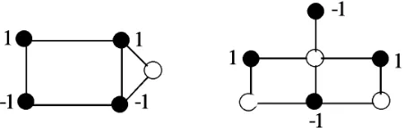
corresponding toxF, thecoreofG. Figure 2.1 shows two graphs, of nullity one, with
the same non-zero partxF ofxbut different cores.
Fig. 2.1.TwoMCs with the same feasible non-zero part(1,1,−1,−1)t of the kernel eigenvector.
P are unique.
This prompts us to ask whether there exist graphs wherex=xF. Indeed such
graphs exist and we call them core graphs. A singular graph, on at least two vertices, with a kernel eigenvector having no zero entries, is said to be acore graph. The core graphs of nullity one, are callednut graphs; the smallest one is of order 7 and size 8 [4]. Note that whereas a core ofGis a subgraph associated with a kernel eigenvector ofG, a core graphF is itself a core ofF.
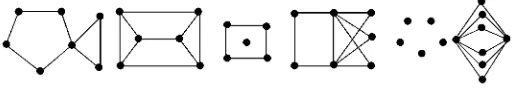
Fig. 2.2.Core Graphs.
Examples of six core graphs in order of increasing nullity, η = 1,2, . . . ,6, are shown in Figure 2.2. For molecular graphs in chemistry, where the vertices represent carbon (C) atoms while the edges represent the C-C sigma bonds, core graphs have a special significance. A radical with the C-structure of a core graph has theπelectronic charge (proportional to the square of the kernel eigenvector entry associated with a C center) occupying the non-bonding orbitals (for λ = 0), distributed all over the carbon centers, and therefore would have markedly different reactivity from the more usual type of radical, where the electron density vanishes at some sites.
2.1. Minimal configurations. The underlying idea, that leads to Definition 2.1 of a MC, is its construction. If, in line with the Interlacing Theorem, to a core graph (F,xF) of nullity η(F)≥1, η(F)−1 independent vertices (forming the periphery),
incident only to vertices of F, can be added, reducing the nullity by one with each vertex addition, then the graphN obtained has nullity one. If we also insist on the condition thatxF remains the non-zero part of the kernel eigenvector ofN, thenN is
a singular graph of nullity one with a minimal number of vertices and edges, having
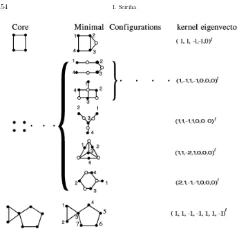
xF as the non-zero part of the kernel eigenvector. Figure 2.3 shows three core graphs.
The MCs grown from the first two, of order four, have a non-empty periphery; the last core graph, of order seven, is a nut graph and hence also a MC.
Definition 2.1. Let F be a core graph on at least two vertices, with nullity
s ≥1 and a kernel eigenvector xF having no zero entries. If a graph N, of nullity
one, havingxF as the non-zero part of the kernel eigenvector, is obtained, by adding
s−1 independent vertices, whose neighbors are vertices ofF, thenN is said to be a
minimal configuration(MC).
Remark 2.2. The allusion to minimality refers to the number of peripheral vertices required to reduce the nullity from η(F) to one, in the construction of N, as well as to the number of edges for N to have core (F,xF). The necessary and
Fig. 2.3.Cores and MCs ‘grown’ from them.
Theorem 2.3. [9] Let N be a singular graph of ordern≥3. The graph N is a
MC having a core(F,xF)and peripheryP :=V(N)−V(F)if and only if the following
conditions are all satisfied:
(i)η(N) = 1,
(ii) P=∅ orP induces a graph consisting of isolated vertices,
(iii)η(F) =|P|+ 1.
Remark 2.4. A MC is connected [9]. In a MC N, a vertex ofP is joined to core-vertices only, N is said to beextendedfrom F and the vertex degree ofv ∈ P is at least two [5]. Note that ifη(G) = 1, thenxF is uniquely determined (up to a
2.2. Singular configurations. For a MC N, if the vertices of F are labeled set of independent vertices whose defining vectors, given by the lasts−1 columns of
N, determine the edges joiningP to the core vertices. Note that if edges are added joining some or all of the distinct pairs of vertices inP, then the graph,S, produced
still satisfiesS
Definition 2.5. A MC, N, and all such graphs, S, are said to be singular configurations(SCs) with underlying spanning MCN.
Proposition 2.6. A SChas nullity one.
Proof. Let S be a SC with spanning MC N. We note fi rst that the kernel eigenvector ofN is also a kernel eigenvector ofS.
IfS=
. Since P corresponds to the zero part ofx, the kernel eigenvector
x=
There remains to show thatS does not have a kernel eigenvector linearly inde-pendent ofx. Indeed, with each addition of a column ofBttoF, the nullity reduces
successively by one. Therefore, there are no linear combinations involving the columns ofBtthat contribute to ker([F Bt]). Since the firstr columns ofS andN are the
same, the only non-zero entries in a kernel eigenvector ofScorrespond to the vertices ofF. ThusS andN share the same unique kernel eigenvector.
The number of SCs with a particular underlying MC,N, is finite and equal to the number of distinct possible ways edges can be inserted joining distinct pairs of vertices of the periphery ofN.
Lemma 2.7. Let N be a MC with periphery P. There exist 2k SCs having the
3. Minimal basis. Let wt(u) denote the weight (that is the number of non-zero entries) of the vector u ∈ Rn. If u1,u2, . . . ,uη are the vectors in a basis
for the nullspace ker(A) of a n×n real matrix A, in non-decreasing weight or-der, such that η
i=1wt(ui) is a minimum, then the basis is said to be a minimal
basis denoted by Bmin. Although various Bmin may be possible, the weight
se-quence {wt(u1),wt(u2), . . . ,wt(uη)} is an invariant for ker(A). Moreover for any
basisB={w1,w2, . . . ,wη}, wt(ui)≤wt(wi) [7].
A basisB for the nullspace can be transformed into another basis B′ by linear
Proposition 3.1. For all possible bases of the nullspace, the set CV of core
vertices is an invariant of a graphG. The core-forbidden vertices,V(G)\CV, are also an invariant of G.
Remark 3.2. The same result holds for the set of vertices corresponding to the non-zero entries of the vectors in the bases for any eigenspace ofG.
This method of constructing MCs by adding a periphery to a core, using the concept that the entries of a kernel eigenvector, corresponding to the periphery, are forced to be zero, was introduced in [5]. A similar idea was also employed in [1], to bound the co-rank of a real symmetric matrix from above.
4. SCs are subgraphs of singular graphs. Henceforth a singular graph with-out isolated vertices will be denoted byH. We show, in Proposition 4.3, that a sin-gular graph of nullityηnecessarily hasηSCs as induced subgraphs and therefore the spanning MCs as subgraphs.
is a SC, which is a vertex-induced subgraph ofH, having xF as the non-zero part of
its kernel eigenvector.
Proof. If the core (F,xF) has core-orderr, then the first r rows ofA(H) may
be partitioned as [F|C] and [F|C]tx
F = 0. Moreover the rank of [F|C] is r−1;
otherwisex in Bmin is equivalent to the linear combination of at least two linearly
independent vectors in the nullspace of A(H), each of which has a smaller weight than x. This would mean that x can be reduced, (using linear combinations with other eigenvectors ofBmin) to another eigenvector of smaller weight that can replace
x in Bmin to produce another basisB′ for ker(A), lexicographically beforeBmin, a
contradiction. If F is not itself a minimal configuration, its nullityµ is more than one. Since row rank and column rank of (A(F)|C) are equal, there exist µ−1 column vectors of the associated matrix Cwhich are linearly independent and form the matrix C′, say, such that A′ = defines the SC,S, grown fromF. The submatrixPof Acorresponds to the entries ofAintersecting in the columns ofC′ and the rows of (C′)t
. Note that the nullity ofA′ is one and the MC spanningS hasP=0. IfF is itself a MC, thenC′ =0and
P(F) =∅; otherwise the successive deletions of the vertices ofP(S), which therefore correspond to the columns ofC′, increase the nullity ofA′by one, with each deletion.
Thusη(F) =|P(N)|+ 1. Noting thatS is an induced subgraph ofH, completes the proof.
Remark 4.2. Since each vector in Bmin corresponds to a unique core and the choice ofxinBminis arbitrary, we have proved the following result on the structure
of singular graphs:
Proposition 4.3. Let H be a singular graph of nullity η. There existη SCs as
Fig. 4.1.MCs are subgraphs of a singular graph.
Example 4.4. An example of a singular graph, of nullity one, is shown in Figure 4.1. The core of the graphG, consists of the six black vertices, that induce the core,
G−7−8, inG. AlthoughGhas nullity one, it is not minimal, since the non-isomorphic graphsG−7 andG−8 are also of nullity one and have the same core asG. These two distinct subgraphs ofGsatisfy the conditions of Theorem 2.3 and are therefore MCs. Moreover,Ghas a kernel eigenvector equal to (1,1,−1,−1,1,−1,0,0) and the vertices 7 and 8, in the periphery, are core-forbidden vertices since they do not lie on any core. For other examples of singular graphs of nullity one where the subgraphs that are possible MCs are neither isomorphic, nor co-spectral, see [11].
Remark 4.5. The need to useBminas a basis becomes clear when one considers a core graph. For instance, the core graphC4k, k≥1, has a kernel eigenvector which
is a linear combination of its twoBmin–vectors but does not have an extension to a
MC withinC4k itself.
4.1. Necessary and sufficient conditions for singularity. We have shown that SCs are admissible induced subgraphs of a singular graphG. Indeed, theη SCs (with spanning MCs) corresponding toBmin may be thought of as the ‘atoms’ ofG.
The graphG may be compared to a ‘molecule’. Carrying the analogy to chemical molecular structure further, we may compare the core of a SC to the ‘nucleus of the atom’ and the periphery to the ‘orbiting electrons’. But ifη SCs with distinct cores are induced subgraphs ofG, isGsingular of nullityη? Since the SCP3is a subgraph
of triangle-free non-singular connected graphs of order three or higher, it is clear that this condition is not sufficient and additional constraints are required.
Lemma 4.6. Let S be aSC having coreF of core-orderpandu= (xF,0, . . . ,0)
be the kernel eigenvector of S (with each of the p entries of xF being non-zero).
Let S be a subgraph of a graph G, labeled such that the first p rows of A(G) are
C′, describes the edges between the vertices of the periphery and those of the core.
Recall thatA(S)u=0. Also the firstprows of A(G) areY =
= 0 and the result follows.
Remark 4.7. Whereas Lemma 4.6 may be considered as a characterization of singular graphs using an algebraic test for singular graphs, the following result is a geometrical criterion for a graph to be singular.
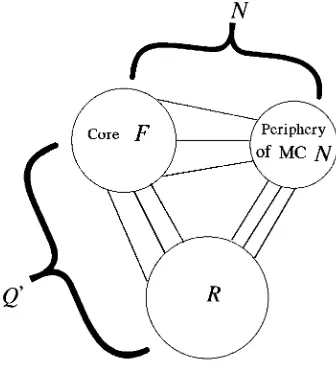
Proposition 4.8. If theSC S with core(F,xF)and periphery P is a subgraph
, then for the same lexicographic ordering of the vertices,
A(F) Q
thatQt
xF=0. Thus,Y t
xF=0, so that (xF,0) is a kernel eigenvector ofG.
We have established a geometrical test which may be considered as a characteri-zation of singular graphs.
Proposition 4.9. A graphG is singular if and only if the following
conditions are both satisfied:
(i) there exists a subgraph of G which is a SC, S, with core (F,xF) and periphery
P =V(S)\V(F);
(ii) the subgraphG− P is also singular with the same core (F,xF).
5. Algorithm. Proposition 4.9 can be utilized iteratively to determine the in-duced SCs for a particular core (F,xF) in a singular graphG(=G0), perhaps with
the use of catalogues of MCs. Lists of the MCs with cores of order less than 6 are found in [5] while in [7], MCs for selected cores of order 6 and 7 are given.
Algorithm:-to determine whether a graph
G
is singular
-to output SCs with common core (
F,
x
F)
and disjoint peripheries.
Step 1: Select an induced SC,Si, with core (F,xF)
and with a partitionV(F) ˙∪Pi of its vertices, inGi−1,
labelling the vertices ofF first. Step 2: ObtainGi by deleting Pi fromGi−1.
Step 3: Incrementiand repeat steps 1 and 2 until no SCs with core (F,xF) remain.
Step4: OutputS:={Si}. IfS =∅, then
(i)Ghas the setS of SCs with core (F,xF);
(ii) andGis singular with a kernel eigenvector (xF,0).
For a large|P|, it becomes easier to notice a SC in the successively smallerG− P, so that implementation of the algorithm becomes progressively less complex. This routine can be repeated for other cores inG.
We conclude with some examples.
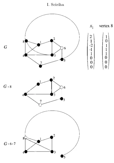
Example 5.1. The graph G in Figure 5.1 has nullity two with 6 as a core-forbidden vertex. The kernel eigenvectors x1 = (2,1,−2,−1,1,0,0,0)t and x2 =
(−1,−1,1,0,0,0,−1,1)tin a minimal basis for the nullspace correspond to the MCs
G−8 and G−5 respectively. Note that the non-isomorphic MCsG−7 andG−8 have a kernel eigenvector with the same feasible non-zero part as x1. Also the
non-isomorphic MCs G−4 and G−5 have a kernel eigenvector with the same feasible non-zero part asx2.
Fig. 5.1. The singular graphG.
We recognize (perhaps by using the catalogue in [5]) thatG−8 is a MC with kernel eigenvector (2,1,−2,−1,1,0,0)t, which isx
1restricted toG−8. Vertex 8 is adjacent
to 1, 3, 4 and 5, so that it has a defining vector v8 = ( 1,0,1,1,1,0,0,0 )
t
. Since
v8 ∈ x1⊥, G is singular with kernel eigenvectorx1, thus completing the algebraic
test.
On the other hand, for the geometric test, we identify the MCG−8 and delete its periphery{6,7}fromG. The subgraphL:=G−6−7 ofG, obtained, is singular with core (F,x1) as required. IndeedLhas nullity two, with two linearly independent
kernel eigenvectors, whose linear combination gives x1. A fundamental system of
cores for L corresponds to MCs P3 and P5 with core-vertices {1,3} and {2,4,5}
respectively.
Example 5.2. Let us now apply the same tests to C6. The 5-vertex path
P5 is a MC with core (F,xF) = (K3,(1,−1,1)t) and is an induced subgraph of the
non-singular graphC6.
For a labeling of the vertices ofC6in cyclic order, vertex 6 is adjacent to 1 and 5,
so that it has a defining vectorv6= ( 1,0,0,0,1,0 )
t
. The kernel eigenvector ofP5 is
(1,0,−1,0,1)t. IfC
eigenvector as P5, then a kernel eigenvector of C6 would be y = (1,0,−1,0,1,0)t.
Since v6 ∈ y⊥, C6 is not singular with core (F,xF). Note that the periphery of
P5 consists of vertices 2 and 4. When these are deleted, the remaining subgraph is
P3∪˙K1, which does not have a core (F,xF). We deduce thatC6 does not have core
(F,xF).
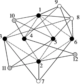
Fig. 5.2.Two SCs with coreK5 and overlapping peripheries.
Example 5.3. The connected graph H in Figure 5.2 has nullity two. The induced subgraphs N1 = H −9 and N2 = H −10 are MCs with the same core
(F,xF) = (K5,(1,1,−1,−1,1)t). Removing the periphery {6,7,8,10} of N1 from
H leaves P3∪3˙ K1 which has core (F,xF). Similarly for N2 which has periphery
{6,7,8,9}. ThusH has two induced SCs, N1 and N2, with core (F,xF) but in this
case, the peripheries are not disjoint. Note that isolated vertices in a core admit any real values as corresponding entries in a kernel eigenvector.
Fig. 5.3.Two SCs with the same coreK2,4 and disjoint peripheries.
Example 5.4. For the connected graph K in Figure 5.3, we apply the above algorithm for a selected core corresponding to aBmin-vector. The nullity ofKis one.
The subgraphS =K− {10,11,12}is a SC. Its core (F,xF) = (K2,4,(−1,1,−3,−1,
2,2)t) induced by the set {1,2,3,4,5,6} of vertices, has nullity four. Removing the
and peripheryP2={10,11,12}. The algorithm outputs the two SCs ofK with core
(F,xF) and disjoint peripheriesP1 andP2.
6. Conclusion. We have seen that SCs are the essential elements of singular graphs. Lemma 4.6 tells us that the presence of a SCSwith core (F,xF) as an induced
subgraph must be complemented by another condition on the edges between F and the vertices of the graph not belonging toS, to ensure that the graph is singular with core (F,xF). Furthermore, Proposition 4.9 provides a geometrical characterization
of singular graphs in terms of admissible induced subgraphs. Having identified a SC with spanning MCN (having core (F,xF) and peripheryP :=VN\VF) as an induced
subgraph of a given graphG, testing the smaller graph G− P not only determines whether Gis singular or otherwise, but also constructs other induced SCs with core (F,xF).
Acknowledgments. The author wishes to thank the Universities of Malta and Messina, the Italian Institute of Culture in Malta and the American Institute of Mathematics, USA, for their support. Sincere thanks go also to the referees for their helpful comments.
REFERENCES
[1] AIM (American Institute of Mathematics) Minimum Rank – Special Graphs Work Group. Zero forcing set and the minumum rank of graphs. Linear Algebra and its Applications, to appear.
[2] H.C. Longuet-Higgins. Some studies in molecular orbital theory I. Resonance structures and molecular orbitals in unsaturated hydrocarbons.Journal of Chemical Physics, 18:265–274, 1950.
[3] A.J. Schwenk and R.J. Wilson. On the eigenvalues of a graph. In L.W. Beineke and R.J. Wilson eds.,Selected Topics in Graph Theory, 307–336, 1978.
[4] I. Sciriha and I. Gutman. Nut graphs – Maximally extending cores. Utilitas Mathematica, 54:257–272, 1998.
[5] I. Sciriha. On the construction of graphs of nullity one. Discrete Mathematics, 181:193–211, 1998.
[6] I. Sciriha. On the coefficient ofλin the characteristic polynomial of singular graphs. Utilitas Mathematica, 52:97–111, 1997.
[7] I. Sciriha. On the rank of graphs. In Y. Alaviet aleds.,The Eighth Quadrennial International Conference on Graph Theory, Combinatorics, Algorithms and Applications, Springer-Verlag, vol. II, 769–778, 1998.
[8] I. Sciriha, S. Fiorini, and J. Lauri. A minimal basis for a vector space.Graph Theory Notes of New York31:21–24, 1996.
[9] I. Sciriha and I. Gutman. Minimal configurations and interlacing.Graph Theory Notes of New York49:38–40, 2005
[10] I. Sciriha and I. Gutman. Minimal configurations trees. Linear and Multilinear Algebra, 54:141–145, 2006.
[11] I. Sciriha and P.W. Fowler. A spectral view of fullerenes. Mathematica Balkanica, 18:183–192, 2004.
[12] L. Spialter. The atom connectivity matrix and its characteristic polynomial.Journal of Chem-ical Documents, 4:261–274, 1964.
[13] R. Wilson. Singular graphs. In V.R. Kulli, ed., Recent Studies in Graph Theory, Vishwa International Publications, 228–236, 1989.