EFFICIENT COMPUTATION OF ENCLOSURES FOR THE EXACT
SOLVENTS OF A QUADRATIC MATRIX EQUATION∗
BEHNAM HASHEMI† AND MEHDI DEHGHAN†
Abstract. None of the usual floating point numerical techniques available for solving the
quadratic matrix equationAX2
+BX+C= 0 with square matricesA, B, CandX, can provide an exact solution; they can just obtain approximations to an exact solution. We use interval arithmetic to compute an interval matrix which contains an exact solution to this quadratic matrix equation, where we aim at obtaining narrow intervals for each entry. We propose a residual version of a modified Krawczyk operator which has a cubic computational complexity, provided thatAis nonsingular and X and X+A−1B
are diagonalizable. For the case thatAis singular or nearly singular, butBis nonsingular we provide an enclosure method analogous to a functional iteration method. Numerical examples have also been given.
Key words. Quadratic matrix equation, Matrix square root, Interval analysis, Krawczyk
oper-ator, Automatic result verification.
AMS subject classifications.65G20, 65F30.
1. Introduction. Many applications such as multivariate rational expectations models [3], noisy Wiener-Hopf problems for Markov chains [11], quasi-birth death process [14], and the quadratic eigenvalue problem
Q(λ)ν = (λ2A+λB+C)ν= 0, λ∈C, ν∈Cn,
(1.1)
which comes from the analysis of damped structural systems, vibration problems [14, 15], and gyroscopic systems [12, 27] require the solution of the quadratic matrix equation
Q(X) =AX2+BX+C= 0.
(1.2)
In (1.2) the known real matricesA, B, Cand the unknown matrixX are of dimension
n×n. A matrixSsatisfyingQ(S) = 0 is called a solvent ofQ(X). The matrix square root problem is a special case of the quadratic matrix equation (1.2). More precisely for A =I, B = 0 andC replaced by−C we haveF(X) =X2−C = 0 and every
square rootS of the matrixC satisfies the equationF(S) = 0.
∗Received by the editors January 21, 2010. Accepted for publication August 16, 2010. Handling
Editor: Daniel B. Szyld.
†Department of Applied Mathematics, Faculty of Mathematics and Computer Sciences,
Amirk-abir University of Technology, No.424 Hafez Avenue, Tehran 15914, Iran (hashemi [email protected], [email protected]).
The quadratic matrix equation (1.2) can have no solvents, a finite positive num-ber, or infinitely many, as follows immediately from the theory of matrix square roots [19]. Suppose thatAis nonsingular in (1.2). ThenQ(λ) in (1.1) has 2neigenvalues, all finite and can be ordered by their absolute values as
|λ1| ≥ |λ2| ≥....≥ |λ2n|.
(1.3)
A solvent S1 of Q(X) is called a dominant solvent if λ(S1) = {λ1, λ2, ..., λn} and
|λn|>|λn+1|, where the eigenvaluesλi ofQ(λ) are ordered as in (1.3). A solventS2
ofQ(X) is called aminimal solventifλ(S2) ={λn+1, λn+2, ..., λ2n}and|λn|>|λn+1|. Theorem 1.1. [19] Assume that the eigenvalues of Q(λ), ordered according to (1.3) satisfy|λn|>|λn+1|and that corresponding to{λi}ni=1 and{λi}2i=nn+1 there are two sets of linearly independent eigenvectors
{ν1, ν2, ..., νn},{νn+1, νn+2, ..., ν2n}.
Then there exists a dominant solvent and a minimal solvent ofQ(X). If, further, the eigenvectors ofQ(λ)are distinct then the dominant and minimal solvents are unique.
Research on the quadratic matrix equation (1.2) goes back at-least to the works by Sylvester in the 1800s [19]. The problem of reducing an algebraic Riccati equa-tion to (1.2) has been analyzed in [4]. Numerical methods for solving (1.2) has been considered including two linearly convergent algorithms for computing a dominant solvent [8, 10]. Davis [6, 7] used Newton’s method for solving (1.2). Kim [19, 20] and Higham and Kim [14, 15] investigated theoretical and numerical results for solving the quadratic matrix equation (1.2). They improved the global convergence properties of Newton’s method with exact line searches and gave a complete characterization of so-lutions in terms of the generalized Schur decomposition. Other numerical techniques, including the functional iteration methods based on Bernoulli’s method, are described and compared in [14]. Recently, Long, Hu and Zhang [23] used Newton’s method with
˘
Samanskii technique to obtain a faster convergence than Newton’s method with exact line searches.
All the above-mentioned numerical techniques rely on floating point arithmetic and thus cannot provide an exact solvent of the quadratic matrix equation (1.2). Indeed, they always obtain only approximations to an exact solvent. In this paper we use interval arithmetic to provide reliable error bounds for each entry of an exact solvent of (1.2). We start with an approximate solvent ˜X, obtained by one of the above-mentioned floating point methods, and aim at computing a tight interval matrix
Hashemi for the matrix square root problem in [9]. Here, we try to generalize the approach of [9] to obtain verified solvents of (1.2).
We assume that the reader is familiar with basic results of interval analysis [2, 26]. The reader can obtain more insight into verified numerical computations based on interval analysis (also called scientific computing with automatic result verification, self-validating methods, or inclusion theory) through hundreds of related publications including many books like [1, 25]. In order to apply techniques of verified numerical computations one needs a correct implementation of machine interval arithmetic. It means that outward rounding has to be applied at each step of a numerical compu-tation on a computer. A website that listed all the interval software is
http://www.cs.utep.edu/intervalcomp/intsoft.html.
An attractive interval arithmetic software is Intlab [32] which is a Matlab toolbox supporting real and complex interval scalars, vectors, and matrices, as well as sparse real and complex interval matrices. Intlab is available online at
http://www.ti3.tu-harburg.de/rump/intlab/.
Another new verification software is Versoft [29] which is a collection of Intlab programs and is freely available at
http://uivtx.cs.cas.cz/~rohn/matlab/index.html.
The organization of this paper is as follows. In Section 2, we introduce our notation and review some basic definitions and concepts. In Section 3 we present the standard Krawczyk operator and show its formulation and difficulties once it has been applied to the quadratic matrix equation (1.2). Section 4 contains our modified Krawczyk operator for enclosing solutions of the quadratic matrix equation (1.2) which dramatically reduces the computational cost of standard Krawczyk operator. In Section 5 we propose a different enclosure method based on a functional iteration method for the case thatAis singular. Section 6 ends this paper with some numerical examples.
2. Notation and preliminary concepts. Throughout this paper lower case letters are used for scalars and vectors and upper case letters for matrices. We use the standard notations of interval analysis [18]. So, all interval quantities will be typeset in boldface. R denotes the field of real numbers, Rn×n the vector space of n×nmatrices with real coefficients,IRthe set of intervals and IRn×n the set of all n×n interval matrices. If x∈ IR, then minx :=xand maxx:= xare the lower
topological interior ofx. We also use the notationICn×nthe set of alln×ncomplex
interval matrices. There are at least two kinds of complex intervals: rectangular intervals and circular intervals [2]. Circular complex interval arithmetic has better algebraic properties than rectangular complex interval arithmetic [2]. We can also implement circular arithmetic completely in terms of BLAS routines to speed up interval computations [31]. This is one of the reasons why Intlab uses circular intervals while working with complex intervals. In this paper we also use circular complex intervals denoted by ICdisc. So, in the remaining part of this paper we use the
convention that each complex interval in IC is represented by a circular interval
in ICdisc. For interval vectors and matrices the above-mentioned operations will
be applied componentwise. Hence, for a complex (real) interval matrix A we can writeA= [midA−radA,mid A+ radA] where midAand radAare the complex (real) center matrix and the complex (real) radius matrix of the interval matrix A, respectively.
For two real matricesA∈Cm×n andB∈Ck×t the Kronecker productA⊗B is
given by themk×nt block matrix
A⊗B=
a11B . . . a1nB
..
. . .. ...
am1B . . . amnB
.
ForA= (aij)∈Cm×n the vector vec(A)∈Cmn is obtained by stacking the columns
of A. We use a convention on the implicit relation between upper and lower case letters when denoting variables, so z = vec(Z), u = vec(U) etc. For an interval matrixA∈ICm×n the vector vec(A) is analogously defined to be an interval vector a= vec(A)∈ICmn.
The Hadamard (pointwise) division of two matricesA, B ∈Cn×m which we
de-note as·/is
A·/B=C∈Cn×m, whereC= (c
ij) withcij =aij/bij.
For d = (d1, . . . , dn)T ∈ Cn, the matrix Diag (d) denotes the diagonal matrix in Cn×n whose i-th diagonal entry is d
i. Also for D ∈ Cn×m we put Diag (D) =
Diag (vec(D)) ∈ Cnm×nm. The following properties of the Kronecker product, vec
operator and Hadamard division will be used several times in this paper.
Lemma 2.1. [16, 9] For real matrices A, B, C and D with compatible sizes we have
The above identities do not hold if we replace the matrices by interval matrices. However, the following enclosure properties are still valid.
Lemma 2.2. [9]Let A,B,C be interval matrices of compatible sizes. Then
{(CT ⊗A)vec(B) :A∈A, B∈B, C∈C} ⊆vec((AB)C).
{(CT ⊗A)vec(B) :A∈A, B∈B, C∈C} ⊆vec(A(BC).
The Fr´echet derivative of a matrix functionG:Cn×n→Cn×n atX ∈Cn×n is a
linear mapping
Cn×n→Cn×n,
E7−→G′ (X)E,
such that for allE∈Cn×n
G(X+E)−G(X)−G′
(X)E=o(||E||),
andG′
(X)E is said to be the Fr´echet derivative ofGapplied to the directionE[13].
3. Standard Krawczyk operator and its use for the quadratic matrix equation (1.2). Letf(x) = 0,f :D⊆Cn→Cn be a nonlinear system of equation
with a continuously differentiable function f, ˜x ∈ Cn, and x ∈ ICn. A mapping S:D×D→Cn×n is called a slope forf if
f(y)−f(x) =S(y, x)(y−x) for allx, y∈D.
LetS be an interval matrix containing all slopesS(y, x) fory∈x. Ifx∈xthe stan-dard choice is S =f′
(x), the interval arithmetic evaluation of f′
(x) which contains the set{f′
(y) :y ∈x}. For real case this follows from the mean-value theorem ap-plied to each componentfi, but for the complex case this is not correct and we cannot
use the mean-value theorem. However, for the complex function under consideration in this paper, we can still enclose slopes by the interval arithmetic evaluation of the derivative. This has been proved in Theorem 3.1 in the following.
Various fixed-point theorems applicable in finite or infinite dimensional spaces, state roughly that, if a mapping maps a set into itself, then that mapping has a fixed-point within that set [17]. For example, the Brouwer fixed-fixed-point theorem states that, if D is homeomorphic to the closed unit ball in Rn and g is a continuous mapping
x=g(x). An interval extensiongofghas the property that, ifxis an interval vector with x ⊆D, then g(x) contains the range {g(x) : x∈ x}. This interval extension once evaluated with outward rounding can be used so that the floating point intervals rigorously contain the actual range ofg. Thus, ifg(x)⊆x, we conclude that ghas a fixed point within x[5, 17, 28].
As a most popular fixed point form forf(x) = 0 one can define
g(x) =x−Rf(x),
(3.1)
whereRis usually taken to be a nonsingular matrix (a nonsingular linear operator in
D ifD is a general linear space [28]). However, it is clear that one can define other fixed point forms forf(x) = 0 depending on the function. Krawczyk interval operator k(˜x,x) is actually based on a mean value extension of the fixed point formgin (3.1). For a given matrixR∈Cn×n, the Krawczyk operatork(˜x,x) defined by
k(˜x,x) = ˜x−Rf(˜x) + (I−R·S)(x−x˜), x˜∈x⊂D.
(3.2)
can then be used to find an enclosures for the solution of the nonlinear system of equationsf(x) = 0. Assume thatS is an interval matrix containing all slopesS(y,˜x) fory∈x. If
k(˜x,x)⊆intx,
(3.3)
then f has a zero x∗
in k(˜x,x). Moreover, if S also contains all slopes S(y, x) for
x, y∈x, the zerox∗
is the only zero off in x[21, 22, 24].
Let us note that the relation (3.3) is likely to hold only if R·S is close to the identity, (i.e.,Ris a good approximation to the inverse of midSwhich is the standard choice for R) and ˜xis a good a good approximation to a zero of f. A method for obtaining trial interval vectorsxaround ˜xfor which the relation (3.3) can be expected to hold is the so-calledǫ-inflation [30].
Let F be the set of floating-point numbers following IEEE standard 754. By A∈Fn×nwe mean thatAis ann×nmatrix with entries that are exactly representable
by a floating-point number in F. In this paper we consider the quadratic matrix
equation (1.2) and suppose thatA, B, C∈Fn×n. The solution matrixXcan, however,
be a matrix inCn×n and we aim at computing enclosures for each entry ofX. The
quadratic matrix equation (1.2) can be reformulated, interpreting matrices as vectors inCn2
viax= vec(X), a= vec(A), b= vec(B), c= vec(C) and using Lemma 2.1 as
q(x) = (XT ⊗A)x+ (I
n⊗B)x+c= 0.
(3.4)
Because
the Fr´echet derivative of the quadratic matrix equation (1.2) at X applied to the directionE is given by
Q′
(X)E=AEX+ (AX+B)E.
Higham and Kim [15] note that if A is nonsingular then Q′
(X) is nonsingular at a dominant or minimal solvent and also at all solventsX if the eigenvalues ofQ(λ) are distinct. By Lemma 2.1, this translates into
q′
(x)e= [XT ⊗A+In⊗(AX+B)]e, andq
′
(x) =XT⊗A+In⊗(AX+B).
Theorem 3.1. Consider the quadratic matrix equation (1.2). Then the interval arithmetic evaluation of the derivative ofq(x), i.e., the interval matrixXT⊗A+I⊗ (AX+B)contains slopes S(y, x)for allx, y∈x.
Proof. Forx, y ∈xwe have
Q(Y)−Q(X) =AY2+BY +C−AX2−BX−C=A(Y2−X2) +B(Y −X)
=1
2A(Y +X)(Y −X) + 1
2A(Y −X)(Y +X) +B(Y −X)
= [1
2A(Y +X) +B](Y −X) + 1
2A(Y −X)(Y +X).
So, using part b) of Lemma 2.1 we have
q(y)−q(x) = [I⊗(1
2A(Y +X) +B)](y−x) + ( 1
2(Y +X)
T ⊗A)(y−x),
which means that
S(y, x) =I⊗[1
2A(Y +X) +B] + 1
2(Y +X)
T⊗A,
is a slope forq. Therefore, forx, y∈x, the slopeS(y, x) is contained in
S(x,x) =I⊗(AX+B) +XT ⊗A,
which is the interval arithmetic evaluation of derivative of the function q(x) = 0.
We note in passing that this theorem also justifies the use of interval arithmetic evaluation of the derivative of the nonlinear function X2−A = 0 for enclosing its
slopes in [9].
The standard Krawczyk operator (3.2) for the particular functionq(x) is given as
k(˜x,x) = ˜x−R( ˜XT ⊗A)˜x+ (In⊗B)˜x+c
[In2−R
midXT⊗A+I⊗(A·midX+B)](x−x˜),
whereR∈Cn2×n2
is an approximate inverse ofq′
(x) = midXT⊗I+I⊗(A·midX+
B). Generally computing such an approximate inverseR requiresO(n6) operations.
On the other hand, then2×n2matrixR does not have a nice Kronecker structure, and it will usually be a full matrix. Each of then2columns of (I⊗(AX+B)+XT⊗A)
hasn2non-zeros. So, computing the product ofRwith (I⊗(AX+B) +XT⊗A) will
requiren4operations for each entry, i.e. a total cost ofO(n6). Overall, the dominant
cost in evaluatingk(˜x,x) isO(n6). Therefore, the main disadvantage of the standard
Krawczyk operator (3.5) for enclosing a solvent of the quadratic matrix equation (1.2) is its huge computational complexity.
So, we need an enclosing method which has been specially designed for the quadratic matrix equation (1.2) and can exploit its structure so that we would be able to obtain an enclosure more cheaply. To our best knowledge there is not any other verification algorithm available in the literature which can be used for the quadratic matrix equation (1.2). The next section is aimed at introducing such an approach.
4. A modified Krawczyk operator for the quadratic matrix equation (1.2). The following slight generalization of (3.3) which expresses the essence of all Krawczyk type verification methods has been proved in [9]. In its formulation we representx as ˜x+z, thus separating the approximate zero ˜xfrom the enclosure of its error,z.
Theorem 4.1. [9]Assume thatf :D⊂Cn→Cn is continuous inD. Letx˜∈D and z ∈ICn be such that x˜+z ⊆D. Moreover, assume that S ⊂Cn×n is a set of matrices containing all slopesS(˜x, y)off for y∈x˜+z=:x. Finally, letR∈Cn×n. Define the setKf(˜x, R,z,S)by
Kf(˜x, R,z,S) :={−Rf(˜x) + (I−RS)z:S∈ S, z∈z}.
(4.1)
Then, if
Kf(˜x, R,z,S)⊆intz,
(4.2)
the function f has a zero x∗
inx˜+Kf(˜x, R,z,S)⊆x. Moreover, if S also contains all slope matricesS(y, x)for x, y∈x, then this zero is unique in x.
We now develop another version of the Krawczyk operator, relying on Theo-rem 4.1, which has a reasonable computational cost of O(n3), provided that A is
nonsingular, and ˜X and ˜X+A−1Bare diagonalizable. The non-singularity condition
Markov chains [11] and for the special case of matrix square roots. Assume that we have the following spectral decompositions forX andX+A−1B
X =VXDXWX, withDX = Diag (λ1, . . . , λn) diagonal, VXWX =I,
(4.3)
and
X+A−1B =V
TDTWT, withDT = Diag (µ1, . . . , µn) diagonal, VTWT =I,
(4.4)
in which VX, DX, WX, VT, DT, WT ∈ Cn×n. Here, VX and VT are the matrices of
right eigenvectors, andWX, WT are the matrices of left eigenvectors.
If X is an accurate approximate solvent of (1.2) then V−1
X XVX and WT(X + A−1B)W−1
T will be close to the diagonal matricesDX andDT, respectively. Because
q′
(x) =XT⊗A+I
n⊗(AX+B) = (In⊗A)· XT ⊗In+In⊗(X+A−1B)=
(In⊗A)·(WXT ⊗VT)· VXTXTV
−T
X ⊗I+I⊗(WT(X+A
−1B)W−1 T )
·(VXT ⊗WT),
an approximate inverse forq′
(x) would be in factorized form
R= (V−T
X ⊗W
−1 T )·∆
−1·(VT
X ⊗WT)·(In⊗A−1),
(4.5)
where ∆ =I⊗DT +DX⊗I. We assume thatVX, WX, DX andVT, WT, DT are
ap-proximated using a floating point method for computing the spectral decompositions (4.3) and (4.4) like MATLAB’seigfunction, So, we do not assume thatVXWX =I
andVTWT =I hold exactly. Moreover, the diagonal matricesDX and DT will
gen-erally not have the exact eigenvalues ofX andT on their diagonal. In other words,
VX, WX, DX and VT, WT, DT are all approximations (not the exact quantities)
ob-tained by a floating point algorithm.
We now introduce Algorithm 1 which by using Part b of Lemma 2.1 efficiently compute
l= vec(L) :=−R·q(x) =−(V−T
X ⊗W
−1 T )∆
−1(VT
X ⊗WT)(In⊗A
−1)·q(x).
Algorithm 1Efficient computation ofl=−Rq(x)
1: ComputeQ=AX2+BX+C 2: ComputeG1=A−1Q
On the other hand we need to compute (I−Rq′
(x))z. For any matrixX ∈Cn×n
and any vectorz∈Cn2 we have
I−R· XT⊗A+I⊗(AX+B)
·z=
(V−T X ⊗W
−1 T )·∆
−1· ∆−I⊗(W
T(X+A−1B)WT−1)−(VX−1XVX)T ⊗I· VXT ⊗WT·z.
The latter expression is rich in Kronecker products, so that using Lemma 2.1 b) we can efficiently computeu= (I−R(XT ⊗A+I⊗(AX+B)))z. See Algorithm 2.
Algorithm 2Efficient computation ofu= (I−Rq′ (x))z
1: ComputeY =WTZVX {Thej-th column ofY will be denotedYj} 2: ComputeS=V−1
X XVX {S is ann×nmatrix with entriesSij} 3: ComputeT =WT(X+A−1B)WT−1
4: fori= 1, . . . , ndo{Compute columnsfi of matrixF}
5: Computefi= (Diag (di)−SiiI−T)Yi{∆ = Diag (D), D= [d1|. . .|dn]∈Cn×n} 6: end for
7: ComputeP =−Y S0+ [f1|. . .|fn] whereS0=S−Diag (S11, . . . , Snn) 8: ComputeN =P·/D
9: ComputeU =W−1 T N V
−1 X
Lines 4-7 in Algorithm 2 compute
p= vec(P) :=
∆−I⊗ WT(X+A
−1B)W−1 T
−(V−1
X XVX)T⊗I
y.
We defined the matrixS0in line 7 of the algorithm so that the diagonal entries of S
are replaced by zeros inS0. The reason for defining S0is to prevent the use of Level 1 BLAS, since machine interval arithmetic as implemented in Intlab is particularly efficient if the Level 2 and Level 3 BLAS are used as much as possible.
We are now in a position to use Algorithm 1 and Algorithm 2 to efficiently com-pute an interval vector containing the setKf(˜x, R,z,S) in (4.1) withf(x) replaced
byq(x)
S =q′
(˜x+z) = ( ˜X+Z)T⊗In+In⊗ A( ˜X+Z)B.
Algorithm 3 obtains an interval vectork= vec(K) = vec(L) + vec(U) containing
Kq(˜x, R,z,q
′
(˜x+z)) ={−Rq(˜x) + (I−RS)z:S∈q′
(˜x+z), z∈z}.
that VX and WT will usually not be available as exact inverses of the computed matrices VX and WT, because they have been obtained using a floating point
algo-rithm. Actually we need to use enclosures for the exact values ofV−1 X andW
−1 T . Such
enclosures can be obtained by using methods of interval analysis like theverifylss
command of Intlab. So, we replaceV−1 X and W
−1
T by interval enclosuresIVX,IWT which we know that contain their exact values, respectively. The same holds for lines 2 and 8 of Algorithm 3, where we replacedA−1by the interval matrixI
A. Note also
that in general for three interval matricesE,F,Gwe have (E·F)·G6=E·(F ·G) because of the subdistributive law of interval arithmetic. But in Algorithm 3 we do not need to indicate the order of interval matrix multiplications; see Lemma 2.2 which guaranteesk ⊇ Kq(˜x, R,z,q′(˜x+z)) for whatever order we choose for the interval
matrix multiplications.
Algorithm 3 Computation of an interval matrix K such that vec(K) contains Kq
with ˜xinstead ofx
1: ComputeQ=A·X˜2+B·X˜+C {Qis an interval matrix due to outward
rounding}
2: ComputeG1=IAQ
3: ComputeG2=WTG1VX {WT andVX are obtained from the spectral
decompositions of ˜X+A−1B and ˜X, respectively} 4: ComputeH=G2·/D
5: ComputeL=−IWTHIVX
6: ComputeY =WTZVX {Thej-th column ofY will be denotedYj} 7: ComputeS=IVX(Z+ ˜X)VX {S is ann×ninterval matrix with entriesSij}
8: ComputeT =WT(Z+ ˜X+IAB)IWT
9: fori= 1, . . . , ndo
10: computefi= (Diag (di)−SiiI−T)Yi 11: end for
12: ComputeP =−Y S0+ [f1|. . .|fn] 13: ComputeN =P ·/D
14: ComputeU =IWTN IVX
15: ComputeK=L+U
The following theorem analyzes the cost of Algorithm 3.
Theorem 4.2. Algorithm 3 requiresO(n3)arithmetic operations.
Proof. Since the main operations in lines 1-8 include interval matrix-matrix mul-tiplications, the computation of Q,G1,G2,H,L,Y,S and T costs O(n3). In lines
9-11, the cost for each i is O(n2), since we have an interval matrix-vector
Since lines 12-15 have also costO(n3), the theorem is proved.
We now use Algorithm 3 to construct our final algorithm that states the use of Krawczyk operator for enclosing an exact solvent of the quadratic matrix equation (1.2). See Algorithm 4.
Algorithm 4 If successful this algorithm provides an interval matrixX containing an exact solvent of the quadratic matrix equation (1.2)
1: Use a floating point algorithm to get an approximate solvent ˜X of (1.2).
{Use Newton’s method with exact line searches, e.g.}
2: Use a floating point algorithm to get approximations for VX, WX, DX and VT, WT, DT in the spectral decomposition of ˜X and ˜X+A−1B, resp.
{Use Matlab’seig, e.g.}
3: Compute interval matrices IVX, IWT and IA containing V −1 X , W
−1
T , and A
−1
resp. {Takeverifylss.mfrom INTLAB, e.g.}
4: ComputeL, an interval matrix containing−Rq(˜x) as in lines 1-5 of Algorithm 3.
5: Z=L
6: fork= 1, . . . kmax do 7: ǫ-inflateZ
8: computeU for input ˜X,Z as in lines 6-14 of Algorithm 3
9: if K:=L+U ⊆intZ then{successful}
10: outputX = ˜X+K andstop
11: else {second try}
12: put Z(2) =Z∩K
13: computeU(2) for input ˜X,Z(2) as in lines 6-14 of Algorithm 3
14: if K(2) =L+U(2)⊆intZ(2) then{successful}
15: outputX = ˜X+K(2) andstop
16: else
17: overwriteZasZ∩K(2)
18: end if
19: end if
20: end for
5. Enclosures based on a functional iteration method in the case that
for the formulation of our algorithms in Section 4. So, in the case that Ais singular or nearly singular, we need an alternative approach.
In Section 3 we noted that Krawczyk interval operators are essentially based on the fixed point function g(x) =x−Rq(x) with q(x) = 0 in (3.4). However, we can define other fixed point functions g for q(x) = 0 in a manner which makes possible the computation of enclosures without inverting the matrix A. In general, given a fixed point equationx=g(x) we can take an interval extension gof gand set up an iterative procedure of the following form [25]
xk+1=g(xk)∩xk : k= 0,1,2, ...
When A in the quadratic matrix equation (1.2) is singular but B is nonsingular, a good choice for the fixed point functiong is
G(X) =−B−1(AX2+C),
i.e.,
g(x) =−(In⊗B
−1) (XT ⊗A)x+c
,
in the vector form. Higham and Kim [14] used the above functionG(X) to construct a functional iteration based on the Bernoulli’s method. The floating point iterative method of [14] is
Xk+1 =−B−1(AXk2+C),
withX0= 0n×n.
If IB is an enclosure for B−1, then G(X) = −IB(AX2+C) is an interval
extension to the functionGin the above. Indeed vec(G(X)) contains the range ofg
overx. We define the following iterative interval scheme
Xk+1=−IB(AX2k+C)∩Xk: k= 0,1,2, ...
(5.1)
If we start with an interval matrixX0 such that G(X0)⊆X0, then (5.1) produces
a nested sequence of interval matrices {Xk} convergent to an interval matrix X∗
which encloses an exact solvent of (1.2) with X∗
= G(X∗
) and X∗
⊆ Xk for all k= 0,1,2, ....
Theorem 5.1.
a) If there exists a solventX∗
of (1.2) inXk, thenX∗∈Xk+1 defined by (5.1). b) If Xk+1 obtained by (5.1) is empty, then there is no solvent of (1.2) inXk. Proof. Firstly suppose that there exists a solventX∗
of (1.2) such thatX∗ ∈Xk.
Then X∗
=G(X∗
) =−B−1(AX∗2
+C)∈ −IB(AX2k+C), i.e.,X
∗
X∗
∈G(Xk)∩Xk, i.e., X∗∈Xk+1.
Now consider second part of theorem and suppose that there is a solvent X∗ of (1.2) inXk. Then the first part of this theorem shows thatX∗ ∈Xk+1 which is a
contradiction. So, the proof is completed.
We emphasize that the iterative method (5.1) cannot be applied to examples with a singular or nearly singular matrixB, like the matrix square root problem which has
B = 0n×n, or the last example in the next section where the condition number ofB
is 1.1×10¹⁸. Another advantage of Algorithm 4 over (5.1) is that different theoretical
and computational aspects of Krawczyk-type methods have been fully analyzed in the literature. For example the choice of an initial interval vector using ǫ-inflation has been a subject of research by itself [30].
As a final remark we note that there are still other possibilities for choosing the fixed point functionGlike
G(X) = (−A−1(BX+C))1/2
(5.2)
as described in [14]. Here, we decided not to work with (5.2), even ifAis nonsingular. The reasons for this are two fold: Firstly, we have Algorithm 4 which works quite well in the case thatAis nonsingular. Secondly, if we want to define an interval iteration by using G(X) = (−A−1(BX +C))1/2, then we need a definition and method of
efficient computation for enclosures for square roots of interval matrices which has not been fully examined in the literature. This can also be a direction for a future research.
6. Numerical experiments. Here we present a comparison of the results ob-tained by the standard Krawczyk operator (3.5) and our modified Krawczyk operator (Algorithm 4). For the special case of matrix square roots there is an alternative algorithm available in thevermatfunroutine of Rohn’s Versoft [29]. But, for the case of quadratic matrix equation (1.2) we could not find any other algorithm to compare with ours. We performed all our experiments on a 2.00 GHz Pentium 4 with 1 GB of RAM. t0 will denote the time spent only for computing the approximation ˜X via Newton’s method with exact line searches andtimewill represent the total computing time, i.e. the time for computing ˜X plus the time needed for the verification. To show the quality of the enclosures obtained, we also report the maximum radiusmrof the components of the enclosing interval matrixX, i.e.
mr=maxn
i,j=1rad (Xij).
So, the value−log10mris the minimum number of correct decimal digits (including
time k mr time k mr
10 0.02 0.10 1 6.3·10−16
0.12 1 3.5·10−15
20 0.06 2.7 1 6.7·10−16
0.21 1 7.6·10−15 40 0.29 145.53 1 7.6·10−16
0.58 1 1.5·10−14 50 0.60 658.42 1 8.1·10−16
1.40 1 1.9·10−14
100 2.50 - - - 5.73 1 4.0·10−14
[image:15.612.64.436.389.479.2]200 18.48 - - - 39.92 1 8.3·10−14
Table 6.1
Results for the damped mass-spring example; all times are in seconds
For the special case of matrix square roots we obtain similar results as those of Algorithm 4 in Table A.1 of [9].
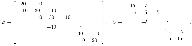
Our first example is a problem given from [14, 19] which arises in a damped mass-spring system with A=In,
B = 20 −10
−10 30 −10
−10 30 −10
−10 . .. . .. 30 −10 −10 20
, C= 15 −5
−5 15 −5
−5 . .. ... . .. ... −5
−5 15 .
Since Newton’s method with exact line searches obtains an approximation to the minimal solvent in this example [14], our algorithms verify existence and uniqueness of the exact value of minimal solvent in a quite narrow interval matrix. Table 6.1 reports the numerical results obtained for different values ofn. An isolated dash (-) in Table 6.1 means that the corresponding test needs more than 15 minutes and we didn’t wait for the standard Krawczyk operator to be completed.
Our second example arises in a quasi-birth-death process with the following ma-trices [14, 19]
A=
0 0.05 0.055 0.08 0.1
0 0 0 0 0
0 0.2 0 0 0
0 0 0.22 0 0
0 0 0 0.32 0.4
, B =
−1 0.01 0.02 0.01 0
0 −1 0 0 0
0 0.04 −1 0 0 0 0 0.08 −1 0 0 0 0 0.04 −1
C=
0.1 0.04 0.025 0.01 0
0.4 0 0 0 0
0 0.16 0 0 0
0 0 0.1 0 0
0 0 0 0.04 0
.
Here, both matricesAandCare singular and so we cannot apply Algorithm 4. Even the standard Krawczyk operator fails to verify the answer. Here, we can use the interval iteration (5.1). Choosing X0 to beintval(zeros(5)); in Intlab notation we obtain after 0.15 seconds an interval matrix withmr= 9.7×10⁻¹⁷. In particular
the elements of the first row of the obtained enclosure are
X11= [0.11186117330535,0.11186117330536],
X12= [0.04596260121747,0.04596260121748],
X13= [0.02710477934505,0.02710477934506],
X14= [0.01026428479283,0.01026428479284],
X15= [0.00000000000000,0.00000000000000].
In our last example we choose A to be the identity matrix, and B and C to be the matricesfrank andgcdmat, respectively. These are matrices from Matlab’s gallery. We set the size of matrices ton= 20. The matrixB is ill-conditioned with a condition number of 1.1×10¹⁸. Both the standard Krawczyk operator and the
iterative scheme (5.1) fail to enclose a solvent. However, Algorithm 4 obtains after 0.8 seconds an enclosure withmr= 2.4×10⁻¹⁰. Here, we see that Algorithm 4 is not
sensitive to the condition ofB, while both the standard Krawczyk method and the iterative method (5.1) need the matrixB to be well-conditioned.
REFERENCES
[1] E. Adams and U. Kulisch. (eds.) Scientific Computing with Automatic Result Verification. Vol. 189 of Mathematics in Science and Engineering, Academic Press Inc., Boston, MA, 1993.
[2] G. Alefeld and J. Herzberger. Introduction to Interval Computations. Computer Science and Applied Mathematics, Academic Press, New York, 1983.
[3] M. Binder and M. Hashem Pesaran. Multivariate rational expectations models and macroe-conometric modelling: A review and some new results. inHandbook of Applied Economet-rics: Macroeconomics. M. Hashem Pesaran and M. Wickens. (eds.), Basil Blackwell, pp. 139–187, 1999.
[4] D. Bini, B. Meini, and F. Poloni. From algebraic Riccati equations to unilateral quadratic matrix equations: old and new algorithms. InDagstuhl Seminar Proceedings 07461, Nu-merical Methods for Structured Markov Chains. 2008.
[5] O. Caprani and K. Madsen. Iterative methods for interval inclusion of fixed points. BIT Numerical Mathematics, 18:42–51, 1978.
[6] G.J. Davis. Numerical solution of a quadratic matrix equation. SIAM Journal on Scientific and Statistical Computing, 2:164–175, 1981.
[7] G.J. Davis. Algorithm 598: An algorithm to compute solvents of the matrix equationAX2 + BX+C= 0. ACM Transactions on Mathematical Software, 9:246–254, 1983.
[8] J.E. Dennis, Jr., J.F. Traub, and R.P. Weber. Algorithms for solvents of matrix polynomials.
SIAM Journal on Numerical Analysis, 15:523–533, 1978.
[9] A. Frommer and B. Hashemi. Verified computation of square roots of a ma-trix. SIAM Journal on Matrix Analysis and Applications, 31:1279–1302, 2009. Preprint available as technical report BUW-SC 09/2, University of Wuppertal,
(www-ai.math.uni-wuppertal.de/SciComp/preprints/SC0902.pdf)
[10] I. Gohberg, P. Lancaster, and L. Rodman. Matrix polynomials. Academic Press Inc. [Harcourt Brace Jovanovich Publishers], New York, 1982. Computer Science and Applied Math-ematics.
[11] C.-H. Guo. On a quadratic matrix equation associated with an M-matrix. IMA Journal of Numerical Analysis, 23:11–27, 2003.
[12] C.-H. Guo. Numerical solution of a quadratic eigenvalue problem. Linear Algebra and its Applications, 385:391–406, 2004.
[13] N.J. Higham. Functions of Matrices: Theory and Computation. SIAM, Philadelphia, 2008. [14] N.J. Higham and H.-M. Kim. Numerical analysis of a quadratic matrix equation.IMA Journal
of Numerical Analysis, 20:499–519, 2000.
[15] N.J. Higham and H.-M. Kim. Solving a quadratric matrix equation by Newton’s method with exact line searches.SIAM Journal on Matrix Analysis and Applications, 23:303–316, 2001. [16] R.A. Horn and C.R. Johnson. Topics in Matrix Analysis. Cambridge University Press,
Cam-bridge, 1994.
[17] R. Kearfott. Interval analysis: Interval fixed point theory. in Encyclopedia of Optimization. Vol. 3, Dordrecht, Netherlands, Kluwer, pp. 45-51, 2001.
[18] R.B. Kearfott, M. Nakao, A. Neumaier, S. Rump, S. Shary, and P. van Hentenryck. Standard-ized notation in interval analysis, 2005.(www.mat.univie.ac.at/~neum/ms/notation.pdf)
[19] H.-M. Kim. Numerical Methods for Solving a Quadratic Matrix Equation. PhD thesis, Uni-versity of Manchester, 2000.
[20] H.-M. Kim. Minimization method for solving a quadratic matrix equation. Kyungpook Math-ematical Journal, 47:239–251, 2007.
[21] R. Krawczyk. Newton-Algorithmen zur Bestimmung von Nullstellen mit Fehlerschranken. Com-puting, 4:187–201, 1969.
forms. SIAM Journal on Numerical Analysis, 22:604–616, 1985.
[23] J.-H. Long, X.-Y. Hu, and L. Zhang. Improved Newton’s method with exact line searches to solve quadratic matrix equation. Journal of Computational and Applied Mathematics, 222:645–654, 2008.
[24] R.E. Moore. A test for existence of solutions to nonlinear systems.SIAM Journal on Numerical Analysis, 14:611–615, 1977.
[25] R.E. Moore, R.B. Kearfott, and M. J. Cloud. Introduction to Interval Analysis. Society for Industrial and Applied Mathematics (SIAM), Philadelphia, PA, 2009.
[26] A. Neumaier. Interval Methods for Systems of Equations. No. 37 in Encyclopedia of Mathe-matics and its Applications, Cambridge University Press, Cambridge, 1990.
[27] J. Qian and W.-W. Lin. A numerical method for quadratic eigenvalue problems of gyroscopic systems. Journal of Sound and Vibration, 306:284–296, 2007.
[28] L.B. Rall. A theory of interval iteration. Proceedings of the American Mathematical Society, 86:625–631, 1982.
[29] J. Rohn. VERSOFT: Verification Software in MATLAB/INTLAB.
(uivtx.cs.cas.cz/~rohn/matlab)
[30] S.M. Rump. A note on epsilon-inflation. Reliable Computing, 4:371–375, 1998.
[31] S.M. Rump. Fast and parallel interval arithmetic. BIT Numerical Mathematics, 39:534–554, 1999.