78
THREE-DIMENSIONAL MODEL FOR COHESIVE SEDIMENT TRANSORT
IN ESTUARY OF PALU RIVER
Mohammad Lutfi
(Staf Pengajar Sekolah Tinggi Teknologi Minyak dan Gas Bumi Balikpapan)
Abstrak
Penelitian ini bertujuan untuk mengkaji dinamika transpor sedimen di Estuari Sungai Palu yang memiliki batimetri curam dan perairan yang dangkal di muara. Simulasi model hidrodinamika dan transpor sedimen dilakukan dengan menggunakan model tiga dimensi ECOMSED yang dibangun oleh HydroQual, Inc., (2002). Simulasi dilakukan dengan menggunakan gaya pembangkit debit sungai dan pasang surut. Hasil simulasi pola arus pada penampang horizontal pada setiap kondisi pasang surut dominan bergerak ke luar teluk, pada penampang vertikal, saat elevasi pasang tertinggi arus bergerak memasuki teluk pada lapisan paling bawah dengan kecepatan arus yang relatif kecil. Perhitungan elevasi permukaan dan kecepatan arus pada penampang vertikal memperlihatkan kesesuaian yang baik dengan data sekunder dan DISHIDROS dan observasi arus. Hasil simulasi transpor sedimen menunjukkan bahwa konsentrasi sedimen pada penampang horizontal dan vertikal dominan dipengaruhi oleh debit sungai dibandingkan dengan pengaruh pasang surut.
Kata Kunci: ECOMSED, Estuari, Kohesif, Palu, dan Sedimen. Palu river estuary region covers most
part of Palu river basin and Palu bay which located in the area of Palu city. Palu river basin has a length of about 102 km with an area of about 339.775 ha. Based on the topographyc map of Palu, it can be estimated that there are about 50 large and small rivers that flow into this river. Palu River is the outlet of all the rivers that flow into Palu river basin with a length of about 42 km.
According to Purwaningsih (2009), Palu River has some problems and strategic issues such as, erosion in the catchment area due to encroachment which causes high fluctuations in the river and sedimentation at the river channel and estuary. The profile of the river can not accommodate the over flow due to sedimentation in the river channel and the river mouth. Sand dredging in the river channel (excavation activity C) has caused an erosion-prone land due to rainwater and floating residential which less pay attention to environmental factors.
One of the three-dimensional numerical models that can be applied to analyze the dynamics of sediment transport and dynamics
of estuarine physical oceanography in the region is a model ECOMSED (Estuary Coastal Ocean Model and Sediment Transport). This model is a state-of-the art hydrodynamic and sediment transport model which realistically computes water circulation, temperature, salinity, mixing and transport, deposition and resuspension of cohesive and non-cohesive sediments (Hydroqual, 2004).
Based on the environmental issues outlined above, the ECOMSED model (in this research) will be applied to analyse cohesive sediment transport dynamics in order to have a good prediction at any time in the future. Modeling of Hydrodynamics
This section explains a relatively detailed description of a numerical circulation module. The module is a three-dimensional coastal ocean model, incorporating to a turbulence closure model to provide a realistic parameterization of the vertical mixing processes. The prognostic variables are the three components of velocity, temperature, salinity, turbulence kinetic energy and turbulence macroscale. The momentum equations are nonlinear and incorporate to a variable Coriolis parameter. Free surface elevation is also calculated prognostically so that the tides and the storm surge events can also be simulated. This is accomplished by means of a splitting mode technique whereby the volume transport and vertical velocity shear are solved separately. The hydrodynamic module described here, is a three-dimensional, time dependent model developed by Blumberg and Mellor (1980, 1987).
The equations that form the basis of the circulation model describe the velocity and surface elevation fields, temperature and salinity fields. Two simplifying approximations are used (Bryan, 1969): first, it is assumed that the weight of the fluid identically balance the pressure (hydrostatic assumption), and second, density differences are neglected unless the differences are multiplied by gravity (Boussinesq approximation).
Consider a system of orthogonal Cartesian coordinates with x increasing to eastward, y increasing to northward, and z increasing to vertically upwards. The free surface located at z = (x, y, t) and the bottom is at z = -H(x, y, t). If V is the horizontal velocity vector with components (U, V) and the horizontal gradient operator, the continuity equation is: situ density, g the gravitational acceleration, P the pressure, and KM the vertical eddy diffusivity of turbulent momentum mixing. A latitudinal variation of the Coriolis parameter,
f, is introduced by use of the plane approximation.
The pressure at depth z can be obtained by integrating the vertical component of the
Patm is assumed constant.
Mohammad Lutfi, Three-Dimensional Model for Cohesive Sediment Transort in Estuary of Palu ……… 80
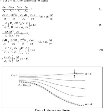
irregularities. It is desirable to introduce a new set of independent variables that transform both the surface and the bottom into coordinate surface (Phillips, 1957) called
-coordinate system which illustrated in Figure 1. The governing external and internal mode
Figure 1. Sigma Coordinate
Note that is the transformed vertical velocity; physically, is the velocity component normal to sigma surfaces. The
D D D
The horizontal viscosity and diffusion terms are defined according to:
ˆ
Modeling of Sediment Transport
The sediment transport module is configured to run in conjunction with the hydrodynamic model and uses the same numerical grid, structure and computational framework as the hydrodynamic model. The sediment dynamic inherent in the model includes sediment resuspension, transport and deposition.
Both resuspension and deposition mechanism depend upon the shear stress induced at the sediment-water interface. Computation of bottom shear stress is an integral part of the sediment transport processes. The resuspension of sediments from the cohesive bed follows the
characteristic equation for resuspension of cohesive sediment, resulting in a certain mass flux of sediments into the water column. Settling of cohesive sediments in the water column is modeled as function of flocculation process.
Sediments forming a cohesive sediment bed consolidate with time. A vertically segmented bed model incorporates the effect of consolidation on the sediment bed properties.
Mohammad Lutfi, Three-Dimensional Model for Cohesive Sediment Transort in Estuary of Palu ……… 82
METHOD
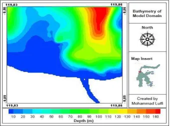
The computational domain of Palu river estuary is shown in Figure 2, which located in the area of 119.8390 to 119.8660 (East Longitude) and from 0.8640 to 0.8920 (South Latitude) or from 816,084.74 to 819,128.97 mT and 9,901,281.95 to 9,904,351.70 mU
The simulation on a vertical cross-section was conducted in the eastern part of the delta, to get an overview of the current dynamics that occured. The site selection was based on the availability of the data for model verification. Location of the simulation was conducted on a vertical cross-section at coordinates 818,205.71 mT, 9.901.910.99 mU till 818,205.71 mT, 9.902.162.61 mU. The depth is divided into 11 layers with different thickness on each layer are as follows: 0.1 m, 0.5 m, 1.0 m, 1.5 m, 2.0 m, 2.5 m, 3.0 m, 4.0 m, 5.0 m and the maximum depth of 167.83 m.
Shoreline data was used as an input data on a closed boundary research area, this data was obtained by digitizing the shoreline on the satélite of IKONOS to identify the image of the coastline between the boundary land and water. Geometric correction was conducted at the IKONOS imagery in year 2005 using topographic maps as a reference
coordinate points. Further geometry correction of the image was obtained from Google Earth image in year 2010 in order to get the actual information about width changes of the river and form changes of the delta in the river mouth.
As a tidal boundary condition, six tide constituents was used as an input data at the boundary of the open sea. This data was needed as tidal generating force by entering its tidal constituents value on the open boundary. The river discharge was used as an open boundary condition at the upstream simulation area. The data was used at the boundary where the water flow into the model.
In this study, the river discharge was assumed to be constant throughout the simulation at 36 m3/s, on the other side, the discharge data of 2 m3/s was needed for verification purpose. At the open boundaries, the sea temperature and salinity was assumed each 290 C and 34 ppt, while the temperature and salinity at the upstream boundary of the river specifically is 280 C and 0 ppt respectively. In the sediment transport model, a constant concentration of 26 mg/L was imposed.in the river boundary was located at the upstream and 1 mg/L was imposed at the sea boundary.
Figure 3. Stages of Geometric Correction
RESULTS AND DISCUSSION
Regional Bathymetry Simulation
The result of the depth interpolation simulation, shows that the simulated model area has a depth that vary with the abruptness in the sea area. The western part is included on the category shallow waters with the depth less than 30 m with a abruptness that is not
too big. While the maximum depth in the northen part is approximately 160 m. In the central and eastern parts show the bathymetric profile with a very large level of abruptness. Abruptness bathymetric depths ranging from 10 m to the maximum depth.
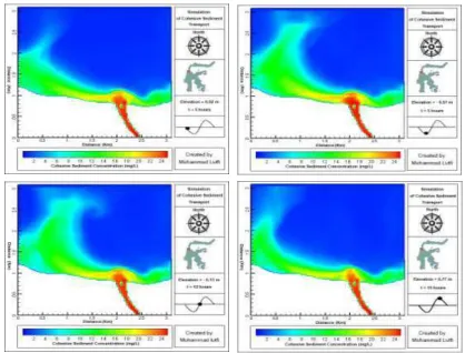
Figure 4. Bathymetry of Model Domain The Patterns of Cohesive Sediment Transport on the Horizontal Cross Section
At the low slack water condition, the concentration of sediment in the upstream area is 26 mg/L. When it reaches the river mouth, the sediment concentration spreads in
Mohammad Lutfi, Three-Dimensional Model for Cohesive Sediment Transort in Estuary of Palu ……… 84
different amount of concentration. The
distribution concentration of cohesive
sediment on the surface in the western part is greater than in the eastern part.
The cause of a larger amount of sediment concentration in the western part than in the eastern part, is caused by the difference of water depth between two locations, thus it will cause more dominant current pattern movements moving to the westward part. Figure 3 shows the bathymetry of the western part is more shallow than the eastern part.
Spatial distribution of sediment at the low slack water condition did not show a
significant changes in the open sea. Changes of the pattern sedimentation only occur in the river mouth. Large sediment concentration in that area is about 26 mg/L. At the flood condition, the spatial distribution of the sediment concentration showed a similar pattern to the low slack water condition. While at the flood condition, the spatial distribution of sediment concentration tend to have a relatively similar pattern to the low slack water condition. The results of the surface sediment transport simulation indicate that the direction of the sediment’s movement follow the current movement patterns.
Figure 5. Cohesive Sediment Concentration in Each Tidal Condition on the Horizontal Cross Section
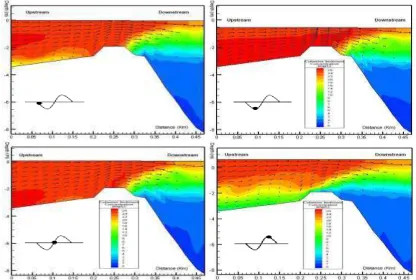
Distribution of Cohesive Sediment Transport on the Vertical Cross Section
Current pattern on the vertical cross section changes at the bottom layer, where the current is generated by tides. It moves from
generated current direction at the bottom layer is in the opposite side of the surface current.
Current velocity decreases with the increasing water depth. At a distance of 0.22 km from the starting point of the simulation area in the middle of the river upstream, the river depth is very shallow and the current velocities are relatively large, which causing the magnitude of cohesive sediment concentration at that location is grow as well. When the low slack water condition, the amount of cohesive sediment concentration varies on each layer, in the middle layer in the upper stream is seen that the relatively large sediment concentration by around 24 mg/L. While in the upper and lower layers respectively is ranged between 22-23 mg/L and 16-20 mg/L.
At ebb conditions, the maximum amount of sediment concentration is ranged between 24-26 mg/L. Current velocity at this condition is relatively large due to the influence of river discharge is also greater
than the effect of tidal. Overall on each layer, the current vector direction moves to the sea with the increasing pace when passing through the shallow areas around the delta, then back down after passing through the delta.
When the tidal current reaches its highest elevation, the current velocity is very small at the bottom of the river. At the bottom layer the current moves into the river. While the upper layer current moving toward the open sea, current velocity gradually reduced at a depth of 2 meters, at a depth of 2 to 3.4 m, moving into the current direction of the river with a relatively large velocity to the open sea, then it gradually began to weaken when the current rate into the river, then increased again when into the shallow area. Cohesive sediment transport simulation result shows that the increasing of the current velocity will increase the greater of the concentration of cohesive sediment transport as well.
Mohammad Lutfi, Three-Dimensional Model for Cohesive Sediment Transort in Estuary of Palu ……… 86
Tidal Verification
Tidal verification was conducted using secondary data on the area tidal of Palu Bay which is obtained by DISHIDROS. This data
is compared with the simulation results of ECOMSED that executed continuously for 16 days (the computing time from the date of July 15 until July 31, 2005).
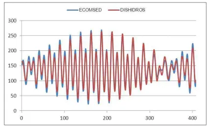
Gambar 7. Comparasion of ECOMSED Simulation Result and Tidal Data DISHIDROS (July 15 until July 31, 2005)
In general, the verification results of the tidal between secondary data of Palu bay with the simulation results by using ECOMSED model in the study área, showed a relatively similar pattern. It can be seen that there is a difference between the tidal amplitude, where the amplitude result simulation is greater than the secondary data from the DISHIDROS data.
In general, the amplitude of the tidal simulation result by using ECOMSED model is smaller than the tidal amplitude which is measured in the real situation on the field. The differentiation of tidal amplitude between ECOMSED simulation and DISHIDROS data are caused by the differences of the data entry of number of tidal constituent (ECOMSED) and tidal prediction (DISHIDROS). Model of ECOMSED requires 6 tidal constituents, namely S2, M2, N2, K1, P1 and O1, while DISHIDROS include 10 constituents tidal
namely M2, S2, N2, K2, K1, O1, P1, M4, MS4 and S0 to predict.
Verification of the Current Velocity on the Vertical Cross Section
The simulation results for the vertical current of 2 m3/s showed a good agreement with the data from field observations (Azizah, 2006). The current velocity at the low slack wáter, ebb, high slack wáter and flood condition, are respectively as follow:
1. At the low slack wáter condition, the simulation results of current velocity ranged from 0 to 0.34 m/s, whereas the observation results ranged from 0 to 0.69 m/s.
3. At the high slack wáter condition, the simulation results of current velocity ranged from 0 to 0.32 m/s, whereas the observation results ranged from 0.94 m/s. 4. At flood condition, the simulation results
of current velocity ranged from 0 to 0.32 m/s, whereas observation results ranged from 0 to 0.72 m/s.
Current velocity differences probably are caused by the differences between the
river’s depth and the discharge in the
upstream area. The river’s depth interpolation on the model ECOMSED was conducted based on the river depth data which is obtained from the Department of Public Works - Palu 2008. As for the observation data is obtained during the field measurement in 2005.
CONCLUSION
The simulation results were conducted by using the river discharge and tide as generating forces, in each tidal condition the current dominantly moved outside the bay, on the vertical cross-section, at high wáter condition goes into the bottom layer with a relatively small current velocity.
The calculation of surface elevation and current velocity on the vertical cross section shows a good agreement with the secondary data from DISHIDROS and the current observation. Sediment concentration on the vertical cross section shows that the Palu river estuary is dominated by the current which is generated by the river discharge.
REFERENCES
Azizah. 2006. Studi Dinamika Estuari Sungai Palu. Skripsi tidak diterbitkan. Palu: Universitas Tadulako..
Blumberg, A.F. 2004. ECOMSED A Three-Dimensional Hydrodynamic and Sediment Transport Model setup & Simulations. USA: HydroQual, Inc. HydroQual, Inc. 2004. A primer for
ECOMSED Version 1.4, Users Manual, Mahwah, N. J. 07430, USA.
Mellor, G. 2004. User Guide for A Theree-Dimensional, Primitive Equation, Numerical Ocean Model, Princeton University. Princeton, NJ 08544-0710. Philips, N.A. 1957. A Coordinate System
Having Some Special Advantages for Numeical Forecasting. J. Meteorol. 14, 184-185.
Purwaningsih. 2009. “Muara Sungai Palu. Melalui”. http://www.radarsulteng. com/berita/index.asp?Berita=Opini&id=4 8759. [05/04/2009].