Seven Databases in Seven Weeks

(1)

(2)

(3)

Seven Databases in Seven Weeks

The flow is perfect. On Friday, you’_{ll be up and running with a new database. On} Saturday, you’_{ll see what it}’_{s like under daily use. By Sunday, you}’_{ll have learned} a few tricks that might even surprise the experts! And next week, you’_{ll vault to} another database and have fun all over again.

➤ _{Ian Dees}

Coauthor, Using JRuby

Provides a great overview of several key databases that will multiply your data modeling options and skills. Read if you want database envy seven times in a row. ➤ _{Sean Copenhaver}

Lead Code Commodore, backgroundchecks.com

This is by far the best substantive overview of modern databases. Unlike the host of tutorials, blog posts, and documentation I have read, this book taught me why I would want to use each type of database and the ways in which I can use them in a way that made me easily understand and retain the information. It was a pleasure to read.

➤ _{Loren Sands-Ramshaw}

Software Engineer, U.S. Department of Defense

This is one of the best CouchDB introductions I have seen. ➤ _{Jan Lehnardt}

(4)

chapter will broaden understanding at all skill levels, from novice to expert— there’_{s something there for everyone.}

➤ _{Jerry Sievert}

Director of Engineering, Daily Insight Group

In an ideal world, the book cover would have been big enough to call this book “_{Everything you never thought you wanted to know about databases that you} can’_{t possibly live without.}”_{To be fair,}_{Seven Databases in Seven Weeks}_will probably sell better.

➤ _{Dr Nic Williams}

(5)

in Seven Weeks

A Guide to Modern Databases

and the NoSQL Movement

Eric Redmond

Jim R. Wilson

The Pragmatic Bookshelf

(6)

Programmers, LLC was aware of a trademark claim, the designations have been printed in initial capital letters or in all capitals. The Pragmatic Starter Kit, The Pragmatic Programmer, Pragmatic Programming, Pragmatic Bookshelf, PragProg and the linking g device are trade-marks of The Pragmatic Programmers, LLC.

Every precaution was taken in the preparation of this book. However, the publisher assumes no responsibility for errors or omissions, or for damages that may result from the use of information (including program listings) contained herein.

Our Pragmatic courses, workshops, and other products can help you and your team create better software and have more fun. For more information, as well as the latest Pragmatic titles, please visit us at http://pragprog.com.

Apache, Apache HBase, Apache CouchDB, HBase, CouchDB, and the HBase and CouchDB logos are trademarks of The Apache Software Foundation. Used with permission. No endorse-ment by The Apache Software Foundation is implied by the use of these marks.

The team that produced this book includes:

Jackie Carter (editor)

Potomac Indexing, LLC (indexer) Kim Wimpsett (copyeditor) David J Kelly (typesetter) Janet Furlow (producer) Juliet Benda (rights) Ellie Callahan (support)

No part of this publication may be reproduced, stored in a retrieval system, or transmitted, in any form, or by any means, electronic, mechanical, photocopying, recording, or otherwise, without the prior consent of the publisher. Printed in the United States of America.

ISBN-13: 978-1-93435-692-0

(7)

Foreword

Riding up the Beaver Run SuperChair in Breckenridge, Colorado, we wondered where the fresh powder was. Breckenridge made snow, and the slopes were immaculately groomed, but there was an inevitable sameness to the conditions on the mountain. Without fresh snow, the total experience was lacking.

In 1994, as an employee of IBM’_{s database development lab in Austin, I had}

very much the same feeling. I had studied object-oriented databases at the University of Texas at Austin because after a decade of relational dominance, I thought that object-oriented databases had a real chance to take root. Still, the next decade brought more of the same relational models as before. I watched dejectedly as Oracle, IBM, and later the open source solutions led by MySQL spread their branches wide, completely blocking out the sun for any sprouting solutions on the fertile floor below.

Over time, the user interfaces changed from green screens to client-server to Internet-based applications, but the coding of the relational layer stretched out to a relentless barrage of sameness, spanning decades of perfectly compe-tent tedium. So, we waited for the fresh blanket of snow.

And then the fresh powder finally came. At first, the dusting wasn’_{t even}

enough to cover this morning’_{s earliest tracks, but the power of the storm}

took over, replenishing the landscape and delivering the perfect skiing expe-rience with the diversity and quality that we craved. Just this past year, I woke up to the realization that the database world, too, is covered with a fresh blanket of snow. Sure, the relational databases are there, and you can get a surprisingly rich experience with open source RDBMS software. You can do clustering, full-text search, and even fuzzy searching. But you’_{re no longer}

limited to that approach. I have not built a fully relational solution in a year.

Over that time, I’_{ve used a document-based database and a couple of}

key-value datastores.

(10)

appropriate models that are simpler, faster, and more reliable. As a person who spent ten years at IBM Austin working on databases with our labs and

customers, this development is simply stunning to me. In Seven Databases

in Seven Weeks, you’_{ll work through examples that cover a beautiful cross}

section of the most critical advances in the databases that back Internet development. Within key-value stores, you’_{ll learn about the radically scalable}

and reliable Riak and the beautiful query mechanisms in Redis. From the columnar database community, you’_{ll sample the power of HBase, a close}

cousin of the relational database models. And from the document-oriented database stores, you’_{ll see the elegant solutions for deeply nested documents}

in the wildly scalable MongoDB. You’_{ll also see Neo4J}’_{s spin on graph}

databases, allowing rapid traversal of relationships.

You won’_{t have to use all of these databases to be a better programmer or}

database admin. As Eric Redmond and Jim Wilson take you on this magical tour, every step will make you smarter and lend the kind of insight that is invaluable in a modern software professional. You will know where each platform shines and where it is the most limited. You will see where your industry is moving and learn the forces driving it there.

Enjoy the ride.

Bruce Tate

author of Seven Languages in Seven Weeks

(11)

Acknowledgments

A book with the size and scope of this one cannot be done by two mere authors alone. It requires the effort of many very smart people with superhuman eyes spotting as many mistakes as possible and providing valuable insights into the details of these technologies.

We’_{d like to thank, in no particular order, all of the folks who provided their}

time and expertise:

Jan Lenhardt Mark Phillips

Ian Dees

Dave Purrington Oleg Bartunov

Robert Stam

Sean Copenhaver Matt Adams

Daniel Bretoi

Andreas Kollegger Emil Eifrem

Loren Sands-Ramshaw

Finally, thanks to Bruce Tate for his experience and guidance.

We’_{d also like to sincerely thank the entire team at the Pragmatic Bookshelf.}

Thanks for entertaining this audacious project and seeing us through it. We’_re

especially grateful to our editor, Jackie Carter. Your patient feedback made this book what it is today. Thanks to the whole team who worked so hard to polish this book and find all of our mistakes.

Last but not least, thanks to Frederic Dumont, Matthew Flower, Rebecca Skinner, and all of our relentless readers. If it weren’_{t for your passion to}

learn, we wouldn’_{t have had this opportunity to serve you.}

For anyone we missed, we hope you’_{ll accept our apologies. Any omissions}

were certainly not intentional.

From Eric: Dear Noelle, you’_{re not special; you}’_{re unique, and that}’_{s so much}

better. Thanks for living through another book. Thanks also to the database creators and commiters for providing us something to write about and make a living at.

From Jim: First, I have to thank my family; Ruthy, your boundless patience

(12)

(13)

Preface

It has been said that data is the new oil. If this is so, then databases are the fields, the refineries, the drills, and the pumps. Data is stored in databases, and if you’_{re interested in tapping into it, then coming to grips with the}

modern equipment is a great start.

Databases are tools; they are the means to an end. Each database has its own story and its own way of looking at the world. The more you understand them, the better you will be at harnessing the latent power in the ever-growing corpus of data at your disposal.

Why Seven Databases

As early as March 2010, we had wanted to write a NoSQL book. The term had been gathering buzz, and although lots of people were talking about it, there seemed to be a fair amount of confusion around it too. What exactly does the

term NoSQL mean? Which types of systems are included? How is this going

to impact the practice of making great software? These were questions we

wanted to answer—_{as much for ourselves as for others.}

After reading Bruce Tate’_{s exemplary}_{Seven Languages in Seven Weeks: A} Pragmatic Guide to Learning Programming Languages [Tat10], we knew he was onto something. The progressive style of introducing languages struck a chord with us. We felt teaching databases in the same manner would provide a smooth medium for tackling some of these tough NoSQL questions.

What

’

s in This Book

This book is aimed at experienced developers who want a well-rounded un-derstanding of the modern database landscape. Prior database experience is not strictly required, but it helps.

(14)

genres or styles, which are discussed in Chapter 1, Introduction, on page 1. In order, they are PostgreSQL, Riak, Apache HBase, MongoDB, Apache CouchDB, Neo4J, and Redis.

Each chapter is designed to be taken as a long weekend’_{s worth of work, split}

up into three days. Each day ends with exercises that expand on the topics and concepts just introduced, and each chapter culminates in a wrap-up discussion that summarizes the good and bad points about the database. You may choose to move a little faster or slower, but it’_{s important to grasp}

each day’_{s concepts before continuing. We}’_{ve tried to craft examples that}

explore each database’_{s distinguishing features. To really understand what}

these databases have to offer, you have to spend some time using them, and that means rolling up your sleeves and doing some work.

Although you may be tempted to skip chapters, we designed this book to be read linearly. Some concepts, such as mapreduce, are introduced in depth in earlier chapters and then skimmed over in later ones. The goal of this book is to attain a solid understanding of the modern database field, so we recom-mend you read them all.

What This Book Is Not

Before reading this book, you should know what it won’_{t cover.}

This Is Not an Installation Guide

Installing the databases in this book is sometimes easy, sometimes challeng-ing, and sometimes downright ugly. For some databases, you’_{ll be able to use}

stock packages, and for others, you’_{ll need to compile from source. We}’_{ll point}

out some useful tips here and there, but by and large you’_{re on your own.}

Cutting out installation steps allows us to pack in more useful examples and a discussion of concepts, which is what you really want anyway, right?

Administration Manual? We Think Not

Along the same lines of installation, this book will not cover everything you’_d

find in an administration manual. Each of these databases has myriad options, settings, switches, and configuration details, most of which are well

document-ed on the Web. We’_{re more interested in teaching you useful concepts and}

full immersion than focusing on the day-to-day operations. Though the

characteristics of the databases can change based on operational settings—

and we may discuss those characteristics—_{we won}’_{t be able to go into all the}

(15)

A Note to Windows Users

This book is inherently about choices, predominantly open source software on *nix platforms. Microsoft environments tend to strive for an integrated environment, which limits many choices to a smaller predefined set. As such, the databases we cover are open source and are developed by (and largely

for) users of *nix systems. This is not our own bias so much as a reflection of the current state of affairs. Consequently, our tutorial-esque examples are presumed to be run in a *nix shell. If you run Windows and want to give it a

try anyway, we recommend setting up Cygwin1 to give you the best shot at

success. You may also want to consider running a Linux virtual machine.

Code Examples and Conventions

This book contains code in a variety of languages. In part, this is a conse-quence of the databases that we cover. We’_{ve attempted to limit our choice}

of languages to Ruby/JRuby and JavaScript. We prefer command-line tools to scripts, but we will introduce other languages to get the job done—_like

PL/pgSQL (Postgres) and Gremlin/Groovy (Neo4J). We’_{ll also explore writing}

some server-side JavaScript applications with Node.js.

Except where noted, code listings are provided in full, usually ready to be executed at your leisure. Samples and snippets are syntax highlighted accord-ing to the rules of the language involved. Shell commands are prefixed by $.

Online Resources

The Pragmatic Bookshelf’_{s page for this book}2_{is a great resource. There you}’_ll

find downloads for all the source code presented in this book. You’_{ll also find}

feedback tools such as a community forum and an errata submission form where you can recommend changes to future releases of the book.

Thanks for coming along with us on this journey through the modern database landscape.

Eric Redmond and Jim R. Wilson

1. http://www.cygwin.com/

(16)

Introduction

This is a pivotal time in the database world. For years the relational model has been the de facto option for problems big and small. We don’_{t expect}

relational databases will fade away anytime soon, but people are emerging from the RDBMS fog to discover alternative options, such as schemaless or alternative data structures, simple replication, high availability, horizontal scaling, and new query methods. These options are collectively known as

NoSQL and make up the bulk of this book.

In this book, we explore seven databases across the spectrum of database styles. In the process of reading the book, you will learn the various function-ality and trade-offs each database has—_{durability vs. speed, absolute vs.}

eventual consistency, and so on—_{and how to make the best decisions for}

your use cases.

1.1 It Starts with a Question

The central question of Seven Databases in Seven Weeks is this: what database or combination of databases best resolves your problem? If you walk away understanding how to make that choice, given your particular needs and resources at hand, we’_{re happy.}

But to answer that question, you’_{ll need to understand your options. For that,}

we’_{ll take you on a deep dive into each of seven databases, uncovering the}

good parts and pointing out the not so good. You’_{ll get your hands dirty with}

CRUD, flex your schema muscles, and find answers to these questions:

• _{What type of datastore is this?}_{Databases come in a variety of genres,}

such as relational, key-value, columnar, document-oriented, and graph. Popular databases—_{including those covered in this book}—_{can generally}

(17)

type and the kinds of problems for which they’_{re best suited. We}’_ve

specifically chosen databases to span these categories including one relational database (Postgres), two key-value stores (Riak, Redis), a col-umn-oriented database (HBase), two document-oriented databases (MongoDB, CouchDB), and a graph database (Neo4J).

• _{What was the driving force?}_{Databases are not created in a vacuum. They}

are designed to solve problems presented by real use cases. RDBMS databases arose in a world where query flexibility was more important than flexible schemas. On the other hand, column-oriented datastores were built to be well suited for storing large amounts of data across sev-eral machines, while data relationships took a backseat. We’_{ll cover cases}

in which to use each database and related examples.

• _{How do you talk to it?}_{Databases often support a variety of connection}

options. Whenever a database has an interactive command-line interface, we’_{ll start with that before moving on to other means. Where programming}

is needed, we’_{ve stuck mostly to Ruby and JavaScript, though a few other}

languages sneak in from time to time—_{like PL/pgSQL (Postgres) and}

Gremlin (Neo4J). At a lower level, we’_{ll discuss protocols like REST}

(CouchDB, Riak) and Thrift (HBase). In the final chapter, we present a more complex database setup tied together by a Node.js JavaScript implementation.

• _{What makes it unique?}_{Any datastore will support writing data and reading}

it back out again. What else it does varies greatly from one to the next. Some allow querying on arbitrary fields. Some provide indexing for rapid lookup. Some support ad hoc queries; for others, queries must be planned. Is schema a rigid framework enforced by the database or merely a set of guidelines to be renegotiated at will? Understanding capabilities and constraints will help you pick the right database for the job.

• _{How does it perform?}_{How does this database function and at what cost?}

Does it support sharding? How about replication? Does it distribute data evenly using consistent hashing, or does it keep like data together? Is this database tuned for reading, writing, or some other operation? How much control do you have over its tuning, if any?

• _{How does it scale?}_{Scalability is related to performance. Talking about}

(18)

whether each datastore is geared more for horizontal scaling (MongoDB, HBase, Riak), traditional vertical scaling (Postgres, Neo4J, Redis), or something in between.

Our goal is not to guide a novice to mastery of any of these databases. A full treatment of any one of them could (and does) fill entire books. But by the end you should have a firm grasp of the strengths of each, as well as how they differ.

1.2 The Genres

Like music, databases can be broadly classified into one or more styles. An individual song may share all of the same notes with other songs, but some are more appropriate for certain uses. Not many people blast Bach’_s_{Mass in} B Minor out an open convertible speeding down the 405. Similarly, some databases are better for some situations over others. The question you must always ask yourself is not “_{Can I use this database to store and refine this}

data?”_{but rather,}“_{Should I?}”

In this section, we’_{re going to explore five main database genres. We}’_{ll also}

take a look at the databases we’_{re going to focus on for each genre.}

It’_{s important to remember that most of the data problems you}’_{ll face could}

be solved by most or all of the databases in this book, not to mention other databases. The question is less about whether a given database style could

be shoehorned to model your data and more about whether it’_{s the best fit}

for your problem space, your usage patterns, and your available resources. You’_{ll learn the art of divining whether a database is intrinsically useful to}

you.

Relational

(19)

There are lots of open source relational databases to choose from, including MySQL, H2, HSQLDB, SQLite, and many others. The one we cover is in

Chapter 2, PostgreSQL, on page 9.

PostgreSQL

Battle-hardened PostgreSQL is by far the oldest and most robust database we cover. With its adherence to the SQL standard, it will feel familiar to anyone who has worked with relational databases before, and it provides a solid point of comparison to the other databases we’_{ll work with. We}’_{ll also explore some}

of SQL’_{s unsung features and Postgres}’_{s specific advantages. There}’_s

some-thing for everyone here, from SQL novice to expert.

Key-Value

The key-value (KV) store is the simplest model we cover. As the name implies, a KV store pairs keys to values in much the same way that a map (or hashtable) would in any popular programming language. Some KV implemen-tations permit complex value types such as hashes or lists, but this is not required. Some KV implementations provide a means of iterating through the keys, but this again is an added bonus. A filesystem could be considered a key-value store, if you think of the file path as the key and the file contents as the value. Because the KV moniker demands so little, databases of this type can be incredibly performant in a number of scenarios but generally

won’_{t be helpful when you have complex query and aggregation needs.}

As with relational databases, many open source options are available. Some of the more popular offerings include memcached (and its cousins mem-cachedb and membase), Voldemort, and the two we cover in this book: Redis and Riak.

Riak

More than a key-value store, Riak—_{covered in}_{Chapter 3,}_Riak_{, on page 51}—

embraces web constructs like HTTP and REST from the ground up. It’_{s a}

faithful implementation of Amazon’_{s Dynamo, with advanced features such}

as vector clocks for conflict resolution. Values in Riak can be anything, from plain text to XML to image data, and relationships between keys are handled by named structures called links. One of the lesser known databases in this book, Riak, is rising in popularity, and it’_{s the first one we}’_{ll talk about that}

(20)

Redis

Redis provides for complex datatypes like sorted sets and hashes, as well as basic message patterns like publish-subscribe and blocking queues. It also has one of the most robust query mechanisms for a KV store. And by caching writes in memory before committing to disk, Redis gains amazing performance in exchange for increased risk of data loss in the case of a hardware failure. This characteristic makes it a good fit for caching noncritical data and for acting as a message broker. We leave it until the end—_see_{Chapter 8,}_Redis_,

on page 261—_{so we can build a multidatabase application with Redis and}

others working together in harmony.

Columnar

Columnar, or column-oriented, databases are so named because the important aspect of their design is that data from a given column (in the two-dimensional table sense) is stored together. By contrast, a row-oriented database (like an RDBMS) keeps information about a row together. The difference may seem inconsequential, but the impact of this design decision runs deep. In column-oriented databases, adding columns is quite inexpensive and is done on a row-by-row basis. Each row can have a different set of columns, or none at all, allowing tables to remain sparse without incurring a storage cost for null values. With respect to structure, columnar is about midway between rela-tional and key-value.

In the columnar database market, there’_{s somewhat less competition than}

in relational databases or key-value stores. The three most popular are HBase (which we cover in Chapter 4, HBase, on page 93), Cassandra, and Hypertable.

HBase

This column-oriented database shares the most similarities with the relational model of all the nonrelational databases we cover. Using Google’_{s BigTable}

paper as a blueprint, HBase is built on Hadoop (a mapreduce engine) and designed for scaling horizontally on clusters of commodity hardware. HBase makes strong consistency guarantees and features tables with rows and

columns—_{which should make SQL fans feel right at home. Out-of-the-box}

support for versioning and compression sets this database apart in the “_Big

Data”_space.

Document

(21)

and so they exhibit a high degree of flexibility, allowing for variable domains. The system imposes few restrictions on incoming data, as long as it meets the basic requirement of being expressible as a document. Different document databases take different approaches with respect to indexing, ad hoc querying, replication, consistency, and other design decisions. Choosing wisely between them requires understanding these differences and how they impact your particular use cases.

The two major open source players in the document database market are MongoDB, which we cover in Chapter 5, MongoDB, on page 135, and CouchDB, covered in Chapter 6, CouchDB, on page 177.

MongoDB

MongoDB is designed to be huge (the name mongo is extracted from the word humongous). Mongo server configurations attempt to remain consistent—_if

you write something, subsequent reads will receive the same value (until the next update). This feature makes it attractive to those coming from an RDBMS background. It also offers atomic read-write operations such as incrementing a value and deep querying of nested document structures. Using JavaScript for its query language, MongoDB supports both simple queries and complex mapreduce jobs.

CouchDB

CouchDB targets a wide variety of deployment scenarios, from the datacenter to the desktop, on down to the smartphone. Written in Erlang, CouchDB has a distinct ruggedness largely lacking in other databases. With nearly incor-ruptible data files, CouchDB remains highly available even in the face of

intermittent connectivity loss or hardware failure. Like Mongo, CouchDB’_s

native query language is JavaScript. Views consist of mapreduce functions, which are stored as documents and replicated between nodes like any other data.

Graph

One of the less commonly used database styles, graph databases excel at dealing with highly interconnected data. A graph database consists of nodes and relationships between nodes. Both nodes and relationships can have properties—_{key-value pairs}—_{that store data. The real strength of graph}

databases is traversing through the nodes by following relationships.

(22)

Neo4J

One operation where other databases often fall flat is crawling through self-referential or otherwise intricately linked data. This is exactly where Neo4J shines. The benefit of using a graph database is the ability to quickly traverse nodes and relationships to find relevant data. Often found in social networking applications, graph databases are gaining traction for their flexibility, with Neo4j as a pinnacle implementation.

Polyglot

In the wild, databases are often used alongside other databases. It’_{s still}

common to find a lone relational database, but over time it is becoming pop-ular to use several databases together, leveraging their strengths to create an ecosystem that is more powerful, capable, and robust than the sum of its parts. This practice is known as polyglot persistence and is a topic we consider further in Chapter 9, Wrapping Up, on page 307.

1.3 Onward and Upward

We’_{re in the midst of a Cambrian explosion of data storage options; it}’_{s hard}

to predict exactly what will evolve next. We can be fairly certain, though, that the pure domination of any particular strategy (relational or otherwise) is unlikely. Instead, we’_{ll see increasingly specialized databases, each suited to}

a particular (but certainly overlapping) set of ideal problem spaces. And just as there are jobs today that call for expertise specifically in administrating relational databases (DBAs), we are going to see the rise of their nonrelational counterparts.

Databases, like programming languages and libraries, are another set of tools that every developer should know. Every good carpenter must understand what’_{s in their toolbelt. And like any good builder, you can never hope to be}

a master without a familiarity of the many options at your disposal.

Consider this a crash course in the workshop. In this book, you’_{ll swing some}

(23)

PostgreSQL

PostgreSQL is the hammer of the database world. It’_{s commonly understood,}

is often readily available, is sturdy, and solves a surprising number of prob-lems if you swing hard enough. No one can hope to be an expert builder without understanding this most common of tools.

PostgreSQL is a relational database management system, which means it’_s

a set-theory-based system, implemented as two-dimensional tables with data rows and strictly enforced column types. Despite the growing interest in newer database trends, the relational style remains the most popular and probably will for quite some time.

The prevalence of relational databases comes not only from their vast toolkits (triggers, stored procedures, advanced indexes), their data safety (via ACID

compliance), or their mind share (many programmers speak and think rela-tionally) but also from their query pliancy. Unlike some other datastores, you needn’_{t know how you plan to use the data. If a relational schema is}

normal-ized, queries are flexible. PostgreSQL is the finest open source example of the

relational database management system (RDBMS) tradition.

2.1 That

’

s Post-greS-Q-L

PostgreSQL is by far the oldest and most battle-tested database in this book. It has plug-ins for natural-language parsing, multidimensional indexing, geographic queries, custom datatypes, and much more. It has sophisticated transaction handling, has built-in stored procedures for a dozen languages, and runs on a variety of platforms. PostgreSQL has built-in Unicode support, sequences, table inheritance, and subselects, and it is one of the most ANSI SQL–_{compliant relational databases on the market. It}’_{s fast and reliable, can}

(24)

So, What

’

s with the Name?

PostgreSQL has existed in the current project incarnation since 1995, but its roots are considerably older. The original project was written at Berkeley in the early 1970s and called the Interactive Graphics and Retrieval System, or “_Ingres”_{for short. In the}

1980s, an improved version was launched post-Ingres—_{shortened to Postgres. The}

project ended at Berkeley proper in 1993 but was picked up again by the open source community as Postgres95. It was later renamed to PostgreSQL in 1996 to denote its rather new SQL support and has remained so ever since.

projects such as Skype, France’_{s Caisse Nationale d}’_{Allocations Familiales}

(CNAF), and the United States’_{Federal Aviation Administration (FAA).}

You can install PostgreSQL in many ways, depending on your operating sys-tem.1 Beyond the basic install, we’_{ll need to extend Postgres with the following}

contributed packages: tablefunc, dict_xsyn, fuzzystrmatch, pg_trgm, and cube. You can refer to the website for installation instructions.2

Once you have Postgres installed, create a schema called book using the fol-lowing command:

$ createdb book

We’_{ll be using the}book_{schema for the remainder of this chapter. Next, run}

the following command to ensure your contrib packages have been installed correctly:

$ psql book -c "SELECT '1'::cube;"

Seek out the online docs for more information if you receive an error message.

2.2 Day 1: Relations, CRUD, and Joins

While we won’_{t assume you}’_{re a relational database expert, we do assume}

you have confronted a database or two in the past. Odds are good that the database was relational. We’_{ll start with creating our own schemas and}

pop-ulating them. Then we’_{ll take a look at querying for values and finally what}

makes relational databases so special: the table join.

Like most databases we’_{ll read about, Postgres provides a back-end server}

that does all of the work and a command-line shell to connect to the running

1. http://www.postgresql.org/download/

(25)

server. The server communicates through port 5432 by default, which you can connect to with the psql shell.

$ psql book

PostgreSQL prompts with the name of the database followed by a hash mark if you run as an administrator and by dollar sign as a regular user. The shell also comes equipped with the best built-in documentation you will find in any console. Typing \h lists information about SQL commands, and \? helps with psql-specific commands, namely, those that begin with a backslash. You can find usage details about each SQL command in the following way:

book=# \h CREATE INDEX

Command: CREATE INDEX

Description: define a new index

Syntax:

CREATE [ UNIQUE ] INDEX [ CONCURRENTLY ] [ name ] ON table [ USING method ]

( { column | ( expression ) } [ opclass ] [ ASC | DESC ] [ NULLS { FIRST | ... [ WITH ( storage_parameter = value [, ... ] ) ]

[ TABLESPACE tablespace ]

[ WHERE predicate ]

Before we dig too deeply into Postgres, it would be good to familiarize yourself with this useful tool. It’_{s worth looking over (or brushing up on) a few common}

commands, like SELECT or CREATE TABLE.

Starting with SQL

PostgreSQL follows the SQL convention of calling relations TABLEs, attributes

COLUMNs, and tuples ROWs. For consistency we will use this terminology, though

you may encounter the mathematical terms relations, attributes, and tuples. For more on these concepts, see Mathematical Relations, on page 12.

Working with Tables

PostgreSQL, being of the relational style, is a design-first datastore. First you design the schema, and then you enter data that conforms to the definition of that schema.

Creating a table consists of giving it a name and a list of columns with types and (optional) constraint information. Each table should also nominate a unique identifier column to pinpoint specific rows. That identifier is called a

PRIMARY KEY. The SQL to create a countries table looks like this:

CREATE TABLE countries (

country_code char(2) PRIMARY KEY, country_name text UNIQUE

(26)

Mathematical Relations

Relational databases are so named because they contain relations (i.e., tables), which are sets of tuples (i.e., rows), which map attributes to atomic values (for example, {name: 'Genghis Khan', p.died_at_age: 65}). The available attributes are defined by a header tuple of attributes mapped to some domain or constraining type (i.e., columns; for example, {name: string, age: int}). That’_{s the gist of the relational structure.}

Implementations are much more practically minded than the names imply, despite sounding so mathematical. So, why bring them up? We’_{re trying to make the point}

that relational databases are relational based on mathematics. They aren’t relational because tables “_relate”_{to each other via foreign keys. Whether any such constraints}

exist is beside the point.

Though much of the math is hidden from you, the power of the model is certainly in the math. This magic allows users to express powerful queries and then lets the system optimize based on predefined patterns. RDBMSs are built atop a set-theory branch called relational algebra—a combination of selections (WHERE ...), projections

(SELECT ...), Cartesian products (JOIN ...), and more, as shown below:

WHERE

SELECT x.name FROM Peoplex x.died_at_age IS NULL

( ( (People))) introduction classes ad infinitum) can cause pain in practice, such as writing code that iterates over all rows. Relational queries are much more declarative than that, springing from a branch of mathematics known as tuple relational calculus, which can be converted to relational algebra. PostgreSQL and other RDBMSs optimize queries by performing this conversion and simplifying the algebra. You can see that the SQL in the diagram below is the same as the previous diagram.

{ t : {name} | x : {name, died_at_age} ( x People x.died_at_age = t.name = x.name )}

free variable result

WHERE

SELECT x.name FROM Peoplex x.died_at_age IS NULL

with attributes name

and died_at_age tuple x is in

relation People and died_at_age

is null and the tuples' attribute name values are equal there exists

a tuple x

(27)

This new table will store a set of rows, where each is identified by a two-character code and the name is unique. These columns both have constraints.

The PRIMARY KEY constrains the country_code column to disallow duplicate country

codes. Only one us and one gb may exist. We explicitly gave country_name a similar unique constraint, although it is not a primary key. We can populate

the countries table by inserting a few rows.

INSERT INTO countries (country_code, country_name)

VALUES ('us','United States'), ('mx','Mexico'), ('au','Australia'),

('gb','United Kingdom'), ('de','Germany'), ('ll','Loompaland');

Let’_{s test our unique constraint. Attempting to add a duplicate}country_name

will cause our unique constraint to fail, thus disallowing insertion. Constraints are how relational databases like PostgreSQL ensure kosher data.

INSERT INTO countries

VALUES ('uk','United Kingdom');

ERROR: duplicate key value violates unique constraint "countries_country_name_key" DETAIL: Key (country_name)=(United Kingdom) already exists.

We can validate that the proper rows were inserted by reading them using

the SELECT...FROM table command.

SELECT *

FROM countries;

country_code | country_name

According to any respectable map, Loompaland isn’_{t a real place}—_let’_{s remove}

it from the table. We specify which row to remove by the WHERE clause. The row whose country_code equals ll will be removed.

DELETE FROM countries

WHERE country_code = 'll';

With only real countries left in the countries table, let’_{s add a}cities_{table. To}

ensure any inserted country_code also exists in our countries table, we add the

REFERENCES keyword. Since the country_code column references another table’_s

(28)

On CRUD

CRUD is a useful mnemonic for remembering the basic data management operations: Create, Read, Update, and Delete. These generally correspond to inserting new records (creating), modifying existing records (updating), and removing records you no longer need (deleting). All of the other operations you use a database for (any crazy query you can dream up) are read operations. If you can CRUD, you can do anything.

CREATE TABLE cities (

name text NOT NULL,

postal_code varchar(9) CHECK (postal_code <> ''), country_code char(2) REFERENCES countries,

PRIMARY KEY (country_code, postal_code)

);

This time, we constrained the name in cities by disallowing NULL values. We constrained postal_code by checking that no values are empty strings (<> means

not equal). Furthermore, since a PRIMARY KEY uniquely identifies a row, we cre-ated a compound key: country_code + postal_code. Together, they uniquely define a row.

Postgres also has a rich set of datatypes. You’_{ve just seen three different string}

representations: text (a string of any length), varchar(9) (a string of variable length up to nine characters), and char(2) (a string of exactly two characters). With our schema in place, let’_{s insert}_{Toronto, CA}_.

INSERT INTO cities

VALUES ('Toronto','M4C1B5','ca');

ERROR: insert or update on table "cities" violates foreign key constraint "cities_country_code_fkey"

DETAIL: Key (country_code)=(ca) is not present in table "countries".

This failure is good! Since country_code REFERENCES countries, the country_code must exist in the countries table. This is called maintaining referential integrity, as in

Figure 1, The REFERENCES keyword constrains fields to another table's pri-mary key, on page 15, and ensures our data is always correct. It’_{s worth}

noting that NULL is valid for cities.country_code, since NULL represents the lack of a value. If you want to disallow a NULL country_code reference, you would define the table cities column like this: country_code char(2) REFERENCES countries NOT NULL.

Now let’_{s try another insert, this time with a U.S. city.}

INSERT INTO cities

VALUES ('Portland','87200','us');

(29)

country_code | country_name

us | United States

mx | Mexico

au | Australia

uk | United Kingdom

de | Germany name | postal_code | country_code

Portland | 97205 | us

Figure 1—The REFERENCES keyword constrains fields to another table’s primary key.

This is a successful insert, to be sure. But we mistakenly entered the wrong

postal_code. The correct postal code for Portland is 97205. Rather than delete

and reinsert the value, we can update it inline.

UPDATE cities

SET postal_code = '97205'

WHERE name = 'Portland';

We have now Created, Read, Updated, and Deleted table rows.

Join Reads

All of the other databases we’_{ll read about in this book perform CRUD}

opera-tions as well. What sets relational databases like PostgreSQL apart is their ability to join tables together when reading them. Joining, in essence, is an operation taking two separate tables and combining them in some way to return a single table. It’_{s somewhat like shuffling up Scrabble pieces from}

existing words to make new words.

The basic form of a join is the inner join. In the simplest form, you specify two columns (one from each table) to match by, using the ON keyword.

SELECT cities.*, country_name

FROM cities INNER JOIN countries

ON cities.country_code = countries.country_code; country_code | name | postal_code | country_name

---+---+---+---us | Portland | 97205 | United States

The join returns a single table, sharing all columns’_{values of the}cities_table

plus the matching country_name value from the countries table.

(30)

A venue exists in both a postal code and a specific country. The foreign key

must be two columns that reference both citiesprimary key columns. (MATCH FULL is a constraint that ensures either both values exist or both are NULL.)

CREATE TABLE venues (

venue_id SERIAL PRIMARY KEY,

name varchar(255),

street_address text,

type char(7) CHECK ( type in ('public','private') ) DEFAULT 'public', postal_code varchar(9),

country_code char(2),

FOREIGN KEY (country_code, postal_code)

REFERENCES cities (country_code, postal_code) MATCH FULL );

This venue_id column is a common primary key setup: automatically increment-ed integers (1, 2, 3, 4, and so on…_{). We make this identifier using the}SERIAL

keyword (MySQL has a similar construct called AUTO_INCREMENT).

INSERT INTO venues (name, postal_code, country_code)

VALUES ('Crystal Ballroom', '97205', 'us');

Although we did not set a venue_id value, creating the row populated it.

Back to our compound join. Joining the venues table with the cities table requires

both foreign key columns. To save on typing, we can alias the table names by following the real table name directly with an alias, with an optional AS between (for example, venues v or venues AS v).

SELECT v.venue_id, v.name, c.name

FROM venues v INNER JOIN cities c

ON v.postal_code=c.postal_code AND v.country_code=c.country_code; venue_id | name | name

---+---+---1 | Crystal Ballroom | Portland

You can optionally request that PostgreSQL return columns after insertion by ending the query with a RETURNING statement.

VALUES ('Voodoo Donuts', '97205', 'us') RETURNING venue_id;

id

-2

(31)

The Outer Limits

In addition to inner joins, PostgreSQL can also perform outer joins. Outer joins are a way of merging two tables when the results of one table must always be returned, whether or not any matching column values exist on the other table.

It’_{s easiest to give an example, but to do that, we}’_{ll create a new table named}

events. This one is up to you. Your events table should have these columns: a

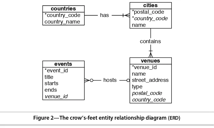
SERIAL integer event_id, a title, starts and ends (of type timestamp), and a venue_id (foreign key that references venues). A schema definition diagram covering all the tables we’_{ve made so far is shown in}_{Figure 2,}_{The crow}_’_{s-feet entity} rela-tionship diagram (ERD), on page 18.

After creating the events table, INSERT the following values (timestamps are inserted as a string like 2012-02-15 17:30), two holidays, and a club we do not talk about.

title | starts | ends | venue_id | event_id

---+---+---+---+---LARP Club | 2012-02-15 17:30:00 | 2012-02-15 19:30:00 | 2 | 1 April Fools Day | 2012-04-01 00:00:00 | 2012-04-01 23:59:00 | | 2 Christmas Day | 2012-12-25 00:00:00 | 2012-12-25 23:59:00 | | 3

Let’_{s first craft a query that returns an event title and venue name as an inner}

join (the word INNER from INNER JOIN is not required, so leave it off here).

SELECT e.title, v.name

FROM events e JOIN venues v

ON e.venue_id = v.venue_id; title | name

---+---LARP Club | Voodoo Donuts

INNER JOIN will return a row only if the column values match. Since we can’_t

have NULL venues.venue_id, the two NULL events.venue_ids refer to nothing. Retrieving all of the events, whether or not they have a venue, requires a LEFT OUTER JOIN (shortened to LEFT JOIN).

SELECT e.title, v.name

FROM events e LEFT JOIN venues v

ON e.venue_id = v.venue_id; title | name

---+---LARP Club | Voodoo Donuts April Fools Day |

(32)

*country_code

Figure 2—The crow’s-feet entity relationship diagram (ERD)

If you require the inverse, all venues and only matching events, use a RIGHT JOIN. Finally, there’_{s the}FULL JOIN_{, which is the union of}LEFT_andRIGHT_{; you}’_re

guaranteed all values from each table, joined wherever columns match.

Fast Lookups with Indexing

The speed of PostgreSQL (and any other RDBMS) lies in its efficient manage-ment of blocks of data, reducing disk reads, query optimization, and other techniques. But those go only so far in fetching results fast. If we select the title of Christmas Day from the events table, the algorithm must scan every

row for a match to return. Without an index, each row must be read from

disk to know whether a query should return it. See the following.

LARP Club | 2 | 1 noticed a message like this:

CREATE TABLE / PRIMARY KEY will create implicit index "events_pkey" \

(33)

PostgreSQL automatically creates an index on the primary key, where the key is the primary key value and where the value points to a row on disk, as shown in the graphic below. Using the UNIQUE keyword is another way to force an index on a table column.

LARP Club | 2 | 1

April Fools Day | | 2

Christmas Day | | 3 1

2

3

"events" Table "events.id" hash Index

SELECT * FROM events WHERE event_id = 2;

You can explicitly add a hash index using the CREATE INDEX command, where

each value must be unique (like a hashtable or a map).

CREATE INDEX events_title

ON events USING hash (title);

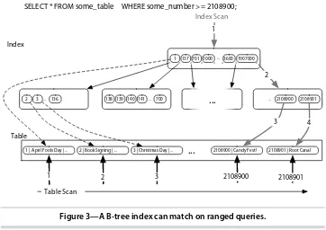
For less-than/greater-than/equals-to matches, we want an index more flexible than a simple hash, like a B-tree (see Figure 3, A B-tree index can match on ranged queries, on page 20). Consider a query to find all events that are on or after April 1.

SELECT *

FROM events

WHERE starts >= '2012-04-01';

For this, a tree is the perfect data structure. To index the starts column with a B-tree, use this:

CREATE INDEX events_starts

ON events USING btree (starts);

Now our query over a range of dates will avoid a full table scan. It makes a huge difference when scanning millions or billions of rows.

We can inspect our work with this command to list all indexes in the schema:

book=# \di

It’_{s worth noting that when you set a}FOREIGN KEY_{constraint, PostgreSQL will}

automatically create an index on the targeted column(s). Even if you don’_t

(34)

1 137 701 1000 ... 3600 1907000

SELECT * FROM some_table WHERE some_number >= 2108900;

Figure 3—A B-tree index can match on ranged queries.

Rails developers), you will often find yourself creating indexes on columns you plan to join against in order to help speed up foreign key joins.

Day 1 Wrap-Up

We sped through a lot today and covered many terms. Here’_{s a recap:}

Definition Term

A domain of values of a certain type, sometimes called an

attribute

Column

An object comprised as a set of column values, sometimes called a tuple

Row

A set of rows with the same columns, sometimes called a relation

Table

The unique value that pinpoints a specific row Primary key

Create, Read, Update, Delete CRUD

Structured Query Language, the lingua franca of a relational database

SQL

Combining two tables into one by some matching columns Join

Combining two tables into one by some matching columns or NULL if nothing matches the left table

(35)

Definition Term

A data structure to optimize selection of a specific set of columns Index

A good standard index; values are stored as a balanced tree data structure; very flexible

B-tree

Relational databases have been the de facto data management strategy for

forty years—_{many of us began our careers in the midst of their evolution. So,}

we took a look at some of the core concepts of the relational model via basic

SQL queries. We will expound on these root concepts tomorrow.

Day 1 Homework

Find

1. Bookmark the online PostgreSQL FAQ and documents. 2. Acquaint yourself with the command-line \? and \h output.

3. In the addresses FOREIGN KEY, find in the docs what MATCH FULL means.

Do

1. Select all the tables we created (and only those) from pg_class. 2. Write a query that finds the country name of the LARP Club event. 3. Alter the venues table to contain a boolean column called active, with the

default value of TRUE.

2.3 Day 2: Advanced Queries, Code, and Rules

Yesterday we saw how to define schemas, populate them with data, update and delete rows, and perform basic reads. Today we’_{ll dig even deeper into}

the myriad ways that PostgreSQL can query data. We’_{ll see how to group}

similar values, execute code on the server, and create custom interfaces using

views and rules. We’_{ll finish the day by using one of PostgreSQL}’_{s contributed}

packages to flip tables on their heads.

Aggregate Functions

An aggregate query groups results from several rows by some common criteria. It can be as simple as counting the number of rows in a table or calculating

the average of some numerical column. They’_{re powerful SQL tools and also}

a lot of fun.

Let’_{s try some aggregate functions, but first we}’_{ll need some more data in our}

database. Enter your own country into the countries table, your own city into

the cities table, and your own address as a venue (which we just named My

(36)

Here’_{s a quick SQL tip: rather than setting the}venue_id_{explicitly, you can}

sub-SELECT it using a more human-readable title. If Moby is playing at the

Crystal Ballroom, set the venue_id like this:

INSERT INTO events (title, starts, ends, venue_id)

VALUES ('Moby', '2012-02-06 21:00', '2012-02-06 23:00', (

SELECT venue_id

FROM venues

WHERE name = 'Crystal Ballroom'

) );

Populate your events table with the following data (to enter Valentine’s Day

in PostgreSQL, you can escape the apostrophe with two, such as Heaven”s

Gate):

title | starts | ends | venue

---+---+---+---Wedding | 2012-02-26 21:00:00 | 2012-02-26 23:00:00 | Voodoo Donuts Dinner with Mom | 2012-02-26 18:00:00 | 2012-02-26 20:30:00 | My Place Valentine’s Day | 2012-02-14 00:00:00 | 2012-02-14 23:59:00 |

With our data set up, let’_{s try some aggregate queries. The simplest aggregate}

function is count(), which is fairly self-explanatory. Counting all titles that contain the word Day (note: % is a wildcard on LIKE searches), you should receive a value of 3.

SELECT count(title)

FROM events

WHERE title LIKE '%Day%';

To get the first start time and last end time of all events at the Crystal Ball-room, use min() (return the smallest value) and max() (return the largest value).

SELECT min(starts), max(ends)

FROM events INNER JOIN venues

ON events.venue_id = venues.venue_id

WHERE venues.name = 'Crystal Ballroom';

min | max

---+---2012-02-06 21:00:00 | ---+---2012-02-06 23:00:00

Aggregate functions are useful but limited on their own. If we wanted to count all events at each venue, we could write the following for each venue ID:

SELECT count(*) FROM events WHERE venue_id = 1;

(37)

This would be tedious (intractable even) as the number of venues grows. Enter

the GROUP BY command.

Grouping

GROUP BY is a shortcut for running the previous queries all at once. With GROUP

BY, you tell Postgres to place the rows into groups and then perform some

aggregate function (such as count()) on those groups.

SELECT venue_id, count(*)

FROM events

GROUP BY venue_id;

venue_id | count

---+---1 | 1 2 | 2 3 | 1 | 3

It’_{s a nice list, but can we filter by the}count()_{function? Absolutely. The}GROUP

BY condition has its own filter keyword: HAVING. HAVING is like the WHERE clause, except it can filter by aggregate functions (whereas WHERE cannot).

The following query SELECTs the most popular venues, those with two or more events:

SELECT venue_id

FROM events

GROUP BY venue_id

HAVING count(*) >= 2 AND venue_id IS NOT NULL; venue_id | count

---+---2 | 2

You can use GROUP BY without any aggregate functions. If you call SELECT...

FROM...GROUP BY on one column, you get all unique values.

SELECT venue_id FROM events GROUP BY venue_id;

This kind of grouping is so common that SQL has a shortcut in the DISTINCT

keyword.

SELECT DISTINCT venue_id FROM events;

(38)

GROUP BY in MySQL

If you tried to run a SELECT with columns not defined under a GROUP BY in MySQL, you may be shocked to see that it works. This originally made us question the necessity of window functions. But when we more closely inspected the data MySQL returns, we found it will return only a random row of data along with the count, not all relevant results. Generally, that’_{s not useful (and quite potentially dangerous).}

Window Functions

If you’_{ve done any sort of production work with a relational database in the}

past, you were likely familiar with aggregate queries. They are a common SQL

staple. Window functions, on the other hand, are not quite so common (Post-greSQL is one of the few open source databases to implement them).

Window functions are similar to GROUP BY queries in that they allow you to run aggregate functions across multiple rows. The difference is that they allow you to use built-in aggregate functions without requiring every single field to be grouped to a single row.

If we attempt to select the title column without grouping by it, we can expect an error.

SELECT title, venue_id, count(*)

FROM events

GROUP BY venue_id;

ERROR: column "events.title" must appear in the GROUP BY clause or \ be used in an aggregate function

We are counting up the rows by venue_id, and in the case of LARP Club and

Wedding, we have two titles for a single venue_id. Postgres doesn’_{t know}_which

title to display.

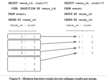
Whereas a GROUP BY clause will return one record per matching group value, a window function can return a separate record for each row. For a visual representation, see Figure 4, Window function results do not collapse results per group, on page 25. Let’_{s see an example of the sweet spot that window}

functions attempt to hit.

Window functions return all matches and replicate the results of any aggregate function.

SELECT title, count(*) OVER (PARTITION BY venue_id) FROM events;

(39)

venue_id | count

1 | 1

2 | 2

3 | 1

| 3

SELECT venue_id, count(*)

OVER (PARTITION BY venue_id)

FROM events

ORDER BY venue_id;

SELECT venue_id, count(*)

FROM events

GROUP BY venue_id

ORDER BY venue_id;

venue_id | count

1 | 1

2 | 2

3 | 1

| 3

Figure 4—Window function results do not collapse results per group.

into fewer rows), it returns grouped values as any other field (calculating on the grouped variable but otherwise just another attribute). Or in SQL parlance, it returns the results of an aggregate function OVER a PARTITION of the result set.

Transactions

Transactions are the bulwark of relational database consistency. All or nothing,

that’_{s the transaction motto. Transactions ensure that every command of a}

set is executed. If anything fails along the way, all of the commands are rolled back like they never happened.

PostgreSQL transactions follow ACID compliance, which stands for Atomic (all ops succeed or none do), Consistent (the data will always be in a good state—_{no inconsistent states), Isolated (transactions don}’_{t interfere), and}

Durable (a committed transaction is safe, even after a server crash). We should note that consistency in ACID is different from consistency in CAP (covered in Appendix 2, The CAP Theorem, on page 317).

(40)

Unavoidable Transactions

Up until now, every command we’ve executed in psql has been implicitly wrapped in

a transaction. If you executed a command, such as DELETE FROM account WHERE total < 20;, and the database crashed halfway through the delete, you wouldn’_{t be stuck with}

half a table. When you restart the database server, that command will be rolled back.

BEGIN TRANSACTION;

DELETE FROM events;

ROLLBACK;

SELECT * FROM events;

The events all remain. Transactions are useful when you’_{re modifying two}

tables that you don’_{t want out of sync. The classic example is a debit/credit}

system for a bank, where money is moved from one account to another:

BEGIN TRANSACTION;

UPDATE account SET total=total+5000.0 WHERE account_id=1337;

UPDATE account SET total=total-5000.0 WHERE account_id=45887;

END;

If something happened between the two updates, this bank just lost five grand. But when wrapped in a transaction block, the initial update is rolled back, even if the server explodes.

Stored Procedures

Every command we’_{ve seen until now has been declarative, but sometimes}

we need to run some code. At this point, you must make a decision: execute code on the client side or execute code on the database side.

Stored procedures can offer huge performance advantages for huge architec-tural costs. You may avoid streaming thousands of rows to a client application, but you have also bound your application code to this database. The decision to use stored procedures should not be arrived at lightly.

Warnings aside, let’_{s create a procedure (or}FUNCTION_{) that simplifies}INSERT_ing

a new event at a venue without needing the venue_id. If the venue doesn’_{t exist,}

create it first and reference it in the new event. Also, we’_{ll return a boolean}

indicating whether a new venue was added, as a nicety to our users.

postgres/add_event.sql

CREATE OR REPLACE FUNCTION add_event( title text, starts timestamp,

ends timestamp, venue text, postal varchar(9), country char(2) )

RETURNS boolean AS $$ DECLARE

(41)

What About Vendor Lock?

When relational databases hit their heyday, they were the Swiss Army knife of tech-nologies. You could store nearly anything—_{even programming entire projects in them}

(for example, Microsoft Access). The few companies that provided this software pro-moted use of proprietary differences and then took advantage of this corporate reliance by charging enormous license and consulting fees. This was the dreaded vendor lock that newer programming methodologies tried to mitigate in the 1990s and early 2000s.

However, in their zeal to neuter the vendors, maxims arose such as no logic in the database. This is a shame because relational databases are capable of so many varied data management options. Vendor lock has not disappeared. Many actions we investigate in this book are highly implementation specific. However, it’_{s worth}

knowing how to use databases to their fullest extent before deciding to skip tools like stored procedures a priori.

found_count integer; the_venue_id integer;

BEGIN

SELECT venue_id INTO the_venue_id

FROM venues v

WHERE v.postal_code=postal AND v.country_code=country AND v.name ILIKE venue

LIMIT 1;

IF the_venue_id IS NULL THEN

VALUES (venue, postal, country)

RETURNING venue_id INTO the_venue_id; did_insert := true;

END IF;

-- Note: not an “error”, as in some programming languages

RAISE NOTICE 'Venue found %', the_venue_id;

INSERT INTO events (title, starts, ends, venue_id)

VALUES (title, starts, ends, the_venue_id);

RETURN did_insert;

END;

$$ LANGUAGE plpgsql;

You can import this external file into the current schema by the following command-line argument (if you don’_{t feel like typing all that code).}

Seven Databases in Seven Weeks