Boundary Conditions for 2D Boussinesq-type Wave-Current
Interaction Equations
Mera, M.1
Abstract: This research focuses on the development of a set of two-dimensional boundary
conditions for specific governing equations. The governing equations are existing Boussinesq-type equations which is capable of simulating wave-current interaction. The present boundary conditions consist of for waves only case and for currents only case. To simulate wave-current interaction, the two kinds of the present boundary conditions are then combined. A numerical model based on both the existing governing equations and the present boundary conditions is applied to simulation of currents only and of wave-current interaction propagating over a basin with a submerged shoal. The results of the numerical model show that the present boundary conditions go well with the existing Boussinesq-type wave-current interaction equations.
Keywords: Boundary condition, Boussinesq, wave, current, free surface.
Introduction
Boussinesq [1] developed the original formulation of the governing equations for a free surface flow, which included the effects of surface waves but in which the vertical dimension was eliminated. The formulation was in terms of the bottom velocity and was restricted to simulating waves moving over bathymetry with a flat bottom. The governing equations consist of one continuity equation and two momentum equations (in x and y directions). The governing equations were then called as Boussinesq equations.
Peregrine [2] developed two new formulations in two horizontal dimensions for the case of varying depth in terms of (i) the depth-averaged velocity vector and (ii) the velocity vector at still water level. The first formulation became known as the standard form of Boussinesq-type equations.
In 1993, Nwogu [3] developed a new approach in the derivation of a novel set of Boussinesq-type equations. The resulting equations are capable of simulating wave propagating over arbitrary bathymetry in terms of the horizontal velocity at an arbitrary level (Z = Z1) below still water level (-h < Z1 < 0) in which h
is the local still water depth. The Boussinesq-type wave equations by Nwogu were solved numerically in one dimension by Nwogu and in two dimensions by Wei and Kirby [4].
1 Civil Engineering, University of Andalas, Padang, INDONESIA
Email: [email protected]
Note: Discussion is expected before June, 1st 2011, and will be
published in the “Civil Engineering Dimension” volume 13, number 2, September 2011.
Received 9 April 2010; revised 6 November; accepted 28 November 2010.
Derivation of two-dimensional (2D) boundary conditions for the governing equations of Nwogu was also discussed by Wei and Kirby.
In 1998, Chen et al. [5] extended the Boussinesq-type wave equations of Nwogu by incorporating a steady ambient current. As a result, the corresponding equations were capable of simulating wave-current interaction. The continuity equation can be expressed as
ηt + ∇•[(h + η) u] + Π= 0 (1)
and the momentum equation is
ut + g∇η + (u•∇)u + Λt + Λs = 0 (2)
where
g = gravitational acceleration
η = free surface elevation
ηt =
t
η ∂ ∂
; ut =
t ∂ ∂u
; Γt =
t ∂
Γ ∂
∇ = ⎟⎟
⎠ ⎞ ⎜⎜
⎝ ⎛
∂ ∂ ∂
∂
y , x
u = horizontal velocity vector, u(x,y,z,t)=(u,v) u = horizontal velocity in the x direction, u(x,y,z,t) v = horizontal velocity in the y direction, v(x,y,z,t)
Π = ∇•(hΓ) – ∇•{1/6 h3∇(∇•u) – 1/2 h2 [∇•(hu)]} +η(h•Γ)
– 1/2η2∇• {∇[∇•(hu)]} – 1/6η3∇•[∇(∇•u)] Γ = 1/2 (Z1)2∇(∇•u) + Z1∇[∇•(hu)]
Λt = Γt – η∇[∇•(hut)] – 1/2η2∇(∇•ut) Λs = (u•∇)Γ – η(u•∇)[∇•(hu)] – 1/2η2(u•∇)[∇(∇•u)]
study. Discussion regarding the numerical solution algorithm is not presented here, but can be found in Mera [6].
Boundary conditions for waves only case
The set of 2D boundary conditions for waves only case is discussed first. The other cases of currents only and waves plus currents will be considered in subsequent sub-section.
Incoming wave boundary conditions
The free surface elevation η at the incoming wave boundary can be varied sinusoidally as
η = 1/2 Hi sin (k•x - ωt) (3)
k•x = (k cos x + (k sin θi) y
In which Hi, is the incoming wave height, k, the wave number vector, x, the horizontal spatial vector,
ω, the angular frequency = 2π/T, T, the wave period, and t is time.
For a locally constant depth, the continuity equation (Eq. 1) reduces to
ηt+ (h + η)(∇•u) + u•∇η + [(α + 1/3) h3 + αh2η – 1/2 hη2
– 1/6 η3] ∇•[∇(∇•u)] = 0 (4)
where
α = 1/2 (Z2)2 + Z2 0.5 < α < 0
Z2 = h
Z1 -1 < Z
2 < 0
A periodic, small amplitude wave can be defined as
η = ηaexp[i(k•x) - ωt], u = ua exp[i(k•x) - ωt] (5)
where:
ηa = amplitude of the water surface elevation;
ua = amplitude of the horizontal velocity vector;
i = -1
θi = incoming wave angle.
Substituting Equation 5 into Equation 4 gives the horizontal velocity vector at the incoming wave boundary, i.e.
u =
}
k{h k [(α / )h αh / h / ]
ω
3 6 1 2 2 1 2 3 3 1
2 η η η
η
− −
+ +
− (6)
Outgoing wave boundary conditions
The boundary condition for η is considered first. At the outgoing wave boundary, the Sommerfeld radiation condition [3] is used to allow the passage and egress of the wave energy, that is
ηt + C •∇η = 0 (7)
where the wave celerity C = |C|cos θi + |C|sin θi.
The boundary condition for the velocity components is considered next. The depth-integrated continuity equation can be expressed in terms of the depth-averaged horizontal velocity vector uas
ηt + ∇• [(h + η)u] = 0 (8)
To eliminate ηt, substitute Equation 8 into the
Sommerfeld radiation condition (Eq. 7) to give
∇• [(h + η)u] = C•∇η (9)
For a locally constant depth, Equation 9 may be integrated over the fluid domain to obtain the horizontal velocity vector
u= C
η η +
h (10)
Having solved for u in Equation 10 is used to determined u.
Reflecting wave boundary conditions
The kinematic boundary condition at an impermeable wall can be stated as
u•n = 0 x∈∂Ω (11)
where n is an outward normal vector, Ω is the fluid domain, ∂Ω is the boundary and x is a position in the boundary. Consider, for example, the case of an impermeable wall being parallel to the x-axis. Equation 11 is a boundary condition and can be written as
v = 0 x∈∂Ω (12)
The slope and the curvature of v normal to the impermeable wall is assumed to be zero and expressed respectively as
0 y v=
∂ ∂
and 0 y
v 2 2
= ∂ ∂
x ∈∂Ω (13)
or can be written symply as
vy = 0 and vyy = 0 x∈∂Ω (14)
in which the subscript y denotes partial differentiation with respect to the y direction
The continuity equation (Eq. 1) can be expressed in terms of the volume flux vector Q as
ηt + ∇•Q = 0 (15) where
Q = (h + η)(u + Γ) – 1/6 (h3 + η3)∇(∇•u) +
1/2 (h2 – η2)∇ [∇•(hu)]
Q•n = 0 x∈∂Ω (16)
For the case of the impermeable wall being parallel to the x-axis, the volume flux in the y-direction at the boundary becomes zero or
Qy= 0 x∈∂Ω (17)
where the subscripts x and y denote partial differentiation with respect to the x and y directions respectively. Substituting Equation 18 into Equation 1 gives a reflecting wave boundary condition for calculating the free surface elevation at the boundary wall as set out below
ηt + [(h + η)u]x + Πx = 0 x∈∂Ω (19)
For a locally constant depth, the horizontal velocity in the x-direction may be obtained by substituting Equations 12 and 13 into Equation 18 giving
uxy = 0 x∈∂Ω (20)
For a boundary being parallel to the x-axis, the boundary conditions are Equations 19, 20 and 12 for
η, u and v respectively. The derivation of the present boundary conditions for waves only case follows Mera [7], who derived a set of boundary conditions for the Boussinesq-type wave equations of Nwogu.
Boundary conditions for currents only case
Inflow Boundary Conditions
At the upstream end, the depth-averaged velocity is specified but the boundary condition also needs to involve η. Inflow currents are bound to flow in the x-direction. One way of linking u and η at the upstream end is to combine the Sommerfeld radiation condition (Eq. 7) and the continuity equation (Eq. 8) to give
2ηt + [(h + η)u]x + Cηx = 0 x∈∂Ω (21)
and
v = 0 x∈∂Ω (22)
Outflow Boundary Conditions
At the downstream end, the free surface elevation can be predicted using Equation 7 in the x direction or
ηt + Cηx = 0 (23)
Then, the horizontal velocities are predicted using Equation 16 in the x direction or
u= C η η
+
h (24)
and in the y direction
v= 0 (25)
No-flow Boundary Conditions
At the boundaries, which are paralel to the flow, the boundary conditions are equivalent to the reflecting wave boundary conditions.
Boundary conditions for wave-current interaction cases
The governing equations considered here were derived based on a steady ambient current. In the model tests, the following procedure is adopted. (1) Model is run with current only.
(2) The results from the model settle down to a steady state.
(3) After the steady state is reached, a sinusoidally varying surface elevation is imposed at the inflow or outflow boundary. This results in a wave train propagating into the computational domain.
Please note that breaking waves are not included in the existing governing equations and in the present boundary conditions considered in this paper. But, Purwanto [8] discussed a Quasi-Equilibrium Turbulent Energy (QETE) model with boundary conditions for breaking and non-breaking waves. The QETE model was intended for simulation of (density) current only case. The density current is a type of current that occurs when fluid flow enters a fluid body of different density.
Numerical set-up
The numerical set-up consists of a basin with a submerged shoal. The basin is 18 m long and 18.2m wide (Figure1). Side walls are at y = 0 and 18.2m. The centre of the shoal was located at (x,y) = (13,9.22) m with the perimeter given by
(x – 13)2 + (y – 9.22)2 = ( 2.57)2 (26)
Wat er surf ace
Side wall Side wall
Current only case
In the first test, a flat water surface (initial value of η = 0) and a steady velocity of 0.10 m/s is imposed at the Southern boundary (x = 0 m). The computation is carried out with a mesh of ∆x = ∆y = 0.1 m and ∆t = 0.02 s. The imposed current flows from x = 0 m to x = 18 m, and reaches a steady state condition after about t = 65 s. Figures 2 shows a perspective view of the free surface elevation (upside down) at t = 65 s predicted by a numerical model based on the existing governing equations of Chen et al. [5] and the present boundary conditions. This figure indicates that the present boundary conditions go well with the existing governing equations.
0
0.0235-0.024 0.023-0.0235 0.0225-0.023 0.022-0.0225 0.0215-0.022 0.021-0.0215 0.0205-0.021 0.02-0.0205 Surface elevation(m):
Current direction
Figure 2. Current only case (flow from x = 0 to x = 18 m).
In the second test, a flat water surface (initial value of η = 0) and a constant inflowing velocity of 0.10 m/s is imposed in the opposite direction to that in first test, i.e. at the Northern boundary (x = 18 m) instead of at the Southern boundary. This leads to a steady current flowing from x = 18 m to x = 0 m of the basin (not presented here).
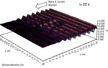
Waves and opposing current
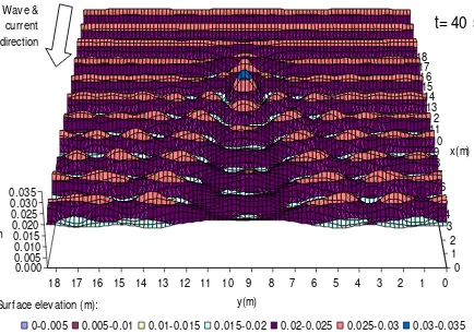
Once the currents in the basin reach a steady state (after about t = 65 s) in the first test, the free surface elevation at the southern boundary (x = 18 m) is sinusoidally varied with time to generate an incident wave. The incoming wave specifications and the grid resolution remain the same as is used in the previous tests i.e.∆x = ∆y = 0.1 m and ∆t = 0.02 s. A wave train with a period of 1.0 s and a wave height of 0.0118 m comes prependicularly to the fluid domain. At the incoming wave boundary (x = 18 m), the ambient current is allowed to pass through, leaving the flow domain. A perspective view of the predicted surface elevation at t = 20 s and at t = 40 s are shown in Figures 3 and 4 respectively. From these figures can be seen that the present boundary conditions are still suitable to the existing governing equations.
0-0.005 0.005-0.01 0.01-0.015 0.015-0.02 0.02-0.025 0.025-0.03 0.03-0.035 0.035-0.04 Surface elevation (m):
Wave direction Current
direction
Figure 3. Waves propagating against a steady, opposing
current at t = 20 s.
0-0.005 0.005-0. 01 0. 01-0. 015 0. 015-0.02 0.02-0.025 0.025-0. 03 0. 03-0. 035 0.035-0.04 Wave
direction
Current direction
Surface elevat ion (m):
Figure 4. Waves propagating against a steady, opposing
current at t = 40.
Waves and current in same direction
On top of the steady current field (second test), a sinusoidal wave train with a period of 1.0 s and a wave height of 0.0118 m is imposed at x = 18 m. The incoming wave period and wave height are same as is used in the last test. Perspective views of the predicted free surface elevation at t = 20 s and at t = 40 s are shown in Figures 5 and 6 respectively in which the present boundary conditions are still going well with the existing governing equations.
0
0-0.005 0.005-0.01 0.01-0.015 0.015-0.02 0.02-0.025 0.025-0.03 0.03-0.035 Surface elevation (m):
Wave & current direction
Figure 5. Waves propagating with a co-flowing steady
0 1 2 3 4 5 6 7 8 9 10 11 12 13 14 15 16 17 18
0 1 2 3 4 5 6 7 8 9 10 11 12 13 14 15 16 17 18
0.000 0.005 0.010 0.015 0.020 0.025 0.030 0.035
m
y(m)
x(m) t= 40 s
0-0.005 0.005-0.01 0.01-0.015 0.015-0.02 0.02-0.025 0.025-0.03 0.03-0.035 Surface elevation (m):
Wave & current direction
Figure 6. Waves propagating with a co-flowing steady
current at t = 40 s.
Conclusions
A set of two-dimensional boundary conditions for the existing Boussinesq-type wave-current interaction equations is developed. The boundary conditions consist of for waves only case and for currents only case. Two kinds of the present boundary conditions are then combined in simulation of wave-current interaction.
A numerical set-up consists of a basin of 18m long and 18.2 m wide with a submerged shoal. The numerical model runs stably at least for 40 s in simulation time as shown by the numerical results. This indicates that the present boundary conditions are suitable to the existing governing equations.
Acknowledgements
The author would like to thanks to Dr. Bruce Cathers from the University of New South Wales for his comments regarding the present material.
References
1. Boussinesq, J., Théorie des ondes et des ramous qui se propagent le long d’un canal rectangulaire horizontal, en communi quant au liquide contenu dans ce canal des vitesses sensiblement pareilles de la surface au fond. J. Math. Pures Appl. 2nd Series 17, 1872, pp. 55-108.
2. Peregrine, D.H., Long Waves on a Beach. J. Fluid Mechanics 27(4), 1967, pp. 815-827.
3. Nwogu, O., Alternative Form of Boussinesq Equations for Nearshore Wave Propagation. J. Waterway Port Coastal and Ocean Eng, ASCE 119(6), 1993, pp. 618-638.
4. Wei, G. and Kirby, J.T., Time-dependent Numerical Code for Extended Boussinesq Equations, J. Waterway Port Coastal and Ocean Eng, ASCE 121(5), 1995, pp. 251-261.
5. Chen, Q., Madsen, P.A., Schäffer, H.A., and Basco, D.R., Wave-current Interaction Based on an Enhanced Boussinesq Approach. Coastal Engineering 33, 1998, pp. 11-39.
6. Mera, M., Boussinesq-type Numerical Models, Ph.D Thesis at the University of New South Wales, Sydney, Australia, 2002.
7. Mera, M., 2D Horizontal Weakly Non-linear Boussinesq-type Numerical Wave Model, Jurnal Teknologi Kelautan, Vol. 11, No. 1, 2007, pp. 37-48.