281
GROUND WATER
7.1 INTRODUCTION
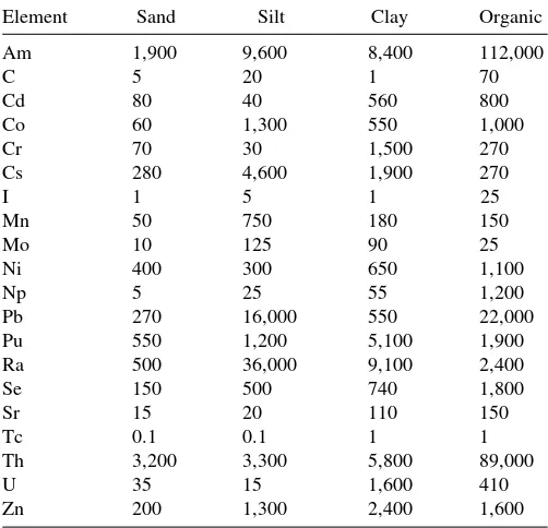
Ground water is a major source of drinking water in the United States, supplying approxi-mately 40% of public water utilities and accounting for almost all of the water supply to rural households (USGS, 1998). It has been estimated that approximately 50% of the U.S. popu-lation relies on ground-water sources for drinking water (Solley et al., 1988). The direct use of ground water for drinking is the reason why drinking-water standards are usually applied to ground water, and the reason why ground-water contamination is such a sensitive issue. A typical ground water contamination scenario is shown in Figure 7.1, where the contami-nant source is located on the ground surface and the contamicontami-nant plume is migrating toward a water-supply well. Ground water frequently contributes the base flow to rivers and streams, a condition that occurs when the river stage is lower than the adjacent water table. Under these conditions, ground-water inflow can contaminate rivers and streams.
Regulations associated with ground-water and wellhead protection programs require engineers to predict the fate and transport of contaminants released either directly into the ground water or on land surfaces above the ground water. These quantitative predictions are used to assess the impact of existing or potential contaminant sources on ground-water quality, to design systems to mitigate any deleterious effects, and to design systems to remediate contaminated ground water.
7.2 NATURAL GROUND-WATER QUALITY
The chemical constituents that occur naturally in ground water enter the aquifer with rainwater through the recharge area, as leachate from the upper soil layer, and from the
dissolution of minerals as the ground water flows through the porous medium. Mineral salts and dissolved (ionized) minerals are the most common sources of natural ground-water quality. The quality of ground ground-water is important since it becomes the base flow of most perennial rivers and streams. The dissolved chemical composition of ground water includes positively charged ions (cations) and negatively charged ions (anions). The most abundant cations in ground water include calcium (Ca2⫹
), iron (Fe2⫹ or Fe3⫹
), magnesium (Mg2⫹
), sodium (Na⫹
), and hydrogen ion acidity (H⫹
). The most abundant negatively charged ions (anions) in ground water include sulfate (SO2
4 ⫺
), nitrate (NO⫺
3), chloride
(Cl⫺
), and bicarbonate (HCO⫺
3). The cations and anions in ground water are balanced
based on their equivalent weight.
Water entering the ground water from atmospheric precipitation is generally acidic (pH⬍7). The normal pH of unpolluted precipitation is 5.6, which is estimated based on the normal saturation vapor pressure of carbon dioxide (CO2) in the atmosphere. Significant atmospheric emissions of acid-forming oxides (SO
2 and NOx) from power
plants, industries, and automobiles can cause the pH of rainfall to be as low as 3. Acid pre-cipitationrefers to precipitation with a pH below 5.6. Production of CO2in the soil by bac-teria can result in pH values of soil and ground water of less than 5. Acidic water entering well-aerated soil reduces some metals from their less soluble forms (e.g., Fe3⫹
) to their more soluble form (e.g., Fe2⫹
). The bicarbonate (HCO⫺
3) content of water in the upper
ground-water zone originates primarily from the dissolution of limestone (CaCO3·nH2O) and dolomite (Ca · MgCO3·nH2O) carbonate minerals as described by the following equi-librium equations:
H2O⫹CO
2⇋H2CO3⇋H ⫹⫹
HCO⫺3
(7.1)
and
CaCO3⫹H
2CO3⇋Ca2 ⫹⫹
2HCO⫺3
(7.2)
Contaminant source
Water-supply well
In more acidic water (pH⬍4.5) the following reaction is more typical:
CaCO3⫹2H ⫹
⇋Ca2⫹⫹H2O⫹CO2 (7.3)
These equations demonstrate the buffering capacity of carbonate materials, which is par-ticularly important in protecting ground water in areas where acid rain occurs. Equations 7.2 and 7.3 further demonstrate that the removal of acidity by limestone and dolomite will increase the hardness of the ground water. Hardness is defined as the content of polyvalent cations, such as Ca2⫹
, Mg2⫹ , Fe2⫹
, and Sr2⫹
expressed on a CaCO3
equiva-lent basis.
Dissolution of minerals is the most important process controlling the quality of ground water. The solubility of minerals and solids is determined by the dissolution–precipitation reaction and their equilibria. A carbonate mineral such as limestone will partially dissolve into its ions as follows:
CaCO3⇋Ca2 ⫹⫹
CO32 ⫺
(7.4)
and the equilibrium in this dissolution–precipitation reaction is given by the reaction equi-librium coefficient,K, given by
K⫽ ᎏ[Ca
where the brackets indicate molar concentrations. The magnitude of the equilibrium coefficient for carbonate minerals indicates a very low solubility in the neutral pH range; however, other minerals, such as salt (NaCl) or gypsum (CaSO4), have relatively high sol-ubility, so that when ground water encounters these layers, high concentrations of Na⫹
, Cl⫺
or Ca2⫹
, and SO42⫺
are common.
Several substances that are normally considered as contaminants at elevated levels occur naturally in ground water and, in some rare instances, the natural levels exceed ground water standards. For example, minerals such as galena may cause elevated levels of lead (Pb). As a further example, Klusman and Edwards (1977) measured toxic metals in ground water from the mineral belt of Colorado and found that drinking-water standards were violated in 14% of the samples for cadmium (Cd) and 9% for zinc (Zn). Other met-als that occur naturally in ground water include antimony, arsenic, beryllium, chromium, copper, lead, mercury, nickel, selenium, silver, and thallium. Table 7.1 lists the natural con-stituents of ground water according to their relative abundance.
7.3 CONTAMINANT SOURCES
7.3.1 Septic Tanks
Septic tanks discharge pathogenic microorganisms, synthetic organic chemicals, nutrients (such as nitrogen and phosphorus), and other contaminants directly into the ground water and can cause serious problems if drinking water sources are too close to the septic tanks. A typical two-chamber septic tank is shown in Figure 7.2. In addition to siting concerns, for septic tanks to work properly it is important that a zone of unsaturated soil exist between the leach bed and the water table so that the effluent from the septic tank does not enter the ground water directly. In the United States, approximately 29% of the population disposes of sewage by individual (on-site) septic systems. Typically, lots using on-site sep-tic systems are rural in nature and utilize their own wells for water supply. Typically, approximately 10% of the water withdrawn from the wells is lost between the well with-drawal and the septic systems through evapotranspiration and consumptive uses such as car washing.
The discharge from septic-tank systems is commonly estimated as 280 L/capita · day, and this effluent typically contains 40 to 80 mg/L of nitrogen, 10 to 30 mg/L of phosphorus,
TABLE 7.1 Typical Natural Constituents of Groundwater
Major Constituents (⬎5 mg/L)
Bicarbonate Chloride Sodium
Carbonic acid Magnesium Sulfate
Calcium Silicon
Minor Constituents (0.1 to 10 mg/L)
Boron Iron Potassium
Carbonate Nitrate Strontium
Fluoride
Trace Constituents (⬍0.1 mg/L)
Aluminum Copper Selenium
Antimony Lead Silver
Arsenic Manganese Thallium
Barium Nickel Thorium
Beryllium Phosphate Uranium
Cadmium Radium Vanadium
Chromium Radon Zinc
Cobalt
Organic Compounds (Shallow Aquifers)
Amino acids Humic acids Tannins
Carbohydrates Hydrocarbons Total organic
Fluvic acids Lignins carbon (TOC)
Organic Compounds (Deep Aquifers)
Acetate Propionate
and 200 to 400 mg/L of BOD5(Sikora et al., 1976; Canter et al., 1987). Based on reported efficiencies of soil absorption systems, the following concentrations are typical of septic-tank effluent entering the ground water (Canter and Knox, 1985): BOD5of 30 to 80 mg/L, COD of 60 to 140 mg/L, ammonia nitrogen of 19 to 80 mg/L, and total phosphorus of 5 to 10 mg/L. Other constituents of concern in septic-tank effluent include bacteria, viruses, nitrates, syn-thetic organics, and toxic metals. Organic matter, BOD5, pathogenic microorganisms, and phosphorus are effectively removed by most properly designed and permitted septic-tank systems, and these contaminants are rarely found more that 1.5 m below the level of dis-charge or beyond the immediate vicinity of the seepage field (Reneau and Petry, 1976; Brown et al., 1979). The nitrification process is typically completed in septic-tank drainfields located in well-drained soils, and the mobile nitrate-nitrogen enters the ground water.
Septic tanks are most likely to contribute to ground-water contamination in areas where (1) there is a high density of homes with septic tanks, (2) the soil layer over permeable bedrock is thin, (3) the soil is extremely permeable, or (4) the water table is less than 1 m below the ground surface.
7.3.2 Leaking Underground Storage Tanks
Underground tanks store gasoline at service stations and are widely used by industry, agri-culture, and homes to store oil, hazardous chemicals, and chemical waste products. A leak-ing underground storage tank is shown in Figure 7.3. Because there are so many underground storage tanks and only a small portion of them are corrosion resistant, the problem of leaking underground storage tanks is a major source of diffuse pollution (Novotny, 2003).
7.3.3 Land Application of Wastewater
Land application of waste sludges and treated wastewater are significant sources of heavy metals, toxic chemicals, and pathogenic microorganisms. A typical wastewater infiltration basin is illustrated in Figure 7.4. There are three types of land application of wastewater: (1) slow-rate systems, (2) overland-flow systems, and (3) rapid infiltration systems. These wastewater systems are described below.
Grade level
Waste Inlet pipe Outlet pipe Effluent
(to tile bed) (from house)
Access cover (manhole)
Scum
Septic tank Sludge
Access cover (manhole)
Effluent
(a) (b)
Slow-rate systems (SRSs) are most common in the United States for treatment of municipal wastewater and effluent reuse in arid areas; in Europe, these systems have been in use for centuries. The hydraulic loading rate for these systems is mostly matched to the irrigation and nutrient requirements for crops and soil permeability. In arid regions, the hydraulic loading is related to the irrigation requirement and prevention of salt buildup in soils. These systems are essentially irrigation systems and have problems similar to those of irrigation return flow and its impact on ground water and base flow. Of the three types
FIGURE 7.3 Leaking underground storage tank. (From USEPA, 2005e.)
of land-application systems, SRSs exhibit the highest nutrient removal due to the com-bined effect of nutrient uptake by crops and attenuation by soils. The disadvantage of low-rate application systems is the large area requirement, typically 30 ha of land per 1000 m3/day of treated sewage.
Inoverland-flow systems(OFSs) wastewater is treated as it moves in graded and main-tained grassed and vegetated sloped areas, and the treated effluent is collected as residual runoffat the bottom of the slope. Percolation of wastewater is not desirable and should be minimized by selection of low-permeability soils, soil compaction, and/or locating these systems over an impermeable subsurface stratum. Under these conditions, the impact of OFSs on ground-water resources should be minimal. OFSs are similar to grassed buffer strips used for treatment of urban and agricultural runoff. Nitrogen removal is accom-plished by nitrification–denitrification processes and depends on the BOD/nitrogen ratio. If the nitrogen in the influent is primarily in nitrate form, the removal is minimal (Reed et al., 1995).
Rapid infiltration systems(RISs) rely on infiltration and filtration of wastewater in per-meable soils. If subsoils are perper-meable, the effluent will reach the ground water and if designed improperly, may become a cause for ground-water contamination. Removal of contaminants in the upper soil layer is accomplished by physical–chemical interaction (adsorption) and biochemical degradation (both aerobic and anaerobic). Vegetation and its nutrient uptake is not considered. If most nitrogen is in nitrate form, removal efficiency is greatly reduced.
Problems associated with land application of wastewater are similar to those for septic tanks; however, much greater volumes of wastewater are concentrated in a smaller area. Mobile pollutants such as nitrates are of greatest concern; other contaminants (BOD, path-ogenic microorganisms, and phosphates) remain near the area of application. Bacteria and viruses die offquite rapidly as wastewater passes through the soil material. The portion of the aquifer that is recharged by treated wastewater effluents should not be used as a source of drinking water and access should be restricted; water should be withdrawn at some safe distance from the recharge area.
Sludge generated by wastewater treatment facilities is commonly applied to agricultural lands as a fertilizer and soil conditioner. The effect of land application of sludge on ground-water quality depends on the transformation that occurs within the topsoil horizon. Although most of the toxic metals will be retained by the topsoil, the toxic metal content of sludge is of concern. Concentrations of toxic metals in wastewater sludge are much higher than those in raw wastewater.
7.3.4 Irrigation and Irrigation Return Flow
Using water that is high in dissolved solids to irrigate an area causes a portion of the irri-gation water to be returned to the atmosphere by evapotranspiration, and since evapotran-spired water has no salt content, there is a subsequent salt and contaminant buildup in soils. The portion returned to the atmosphere may range from less than 20% in high-rate appli-cation systems in humid climatic conditions to almost 100% in low-rate appliappli-cation sys-tems in arid and semiarid climates. Figure 7.5 illustrates irrigation using ground water as a source.
leachate from soils, is either collected by subsurface drainage systems or percolates directly into the ground water. The irrigation water collected by subsurface drainage sys-tems or leached into the ground water is called irrigation return flowand represents one of the more serious problems associated with diffuse pollution of ground water. The con-centration of salts in water percolating through the soil-root level into irrigation return flow or to ground water can be computed using the relation
ciQi⫽caq(Qi⫺Qe) (7.6)
whereciis the salt or contaminant concentration in the water or wastewater used for irri-gation,Qiis the amount of irrigation water also including precipitation that is not lost as surface runoff (⫽effective precipitation),caq is the salt or contaminant concentration of water percolating from the root zone downward, and Qeis the amount of water released from the soil by evapotranspiration. The amount of excess irrigation water that has to be applied to control salt or contaminant buildup in soil depends on the tolerance of a crop to salt in the soil water, the salt content of the irrigation water, evapotranspiration rate, crop uptake, and other losses from the system. The leaching ratio, Qi/Qe, is derived from Equation 7.6:
ᎏ
Q Q
e i ᎏ ⫽ ᎏ
caq c
⫺ aq
ci
ᎏ (7.7)
The salinity of irrigation water is usually expressed as conductivity in microsiemens per centimeter [1000µS/cm⬇640 mg/L of total dissolved solids (TDS)]. The salt tolerance of crops ranges from less than 500µS/cm for salt-sensitive crops such as most fruit trees and some vegetables (celery, strawberries, or beans) to more than 1500 µS/ cm for salt-toler-ant crops such as cotton, beets, barley, and asparagus. Most common grain crops and veg-etables have medium tolerance (500 to 1500µS/ cm) to salts. The leaching requirement (LR) is defined by
where ECiis the electric conductivity of irrigation water and ECaqis the electric conduc-tivity of drainage water. Combining Equations 7.7 and 7.8, the leaching ratiois
ᎏ
Although irrigation return flow has been recognized as a significant water-quality problem, the Clean Water Act in the United States specifically excludes agricultural runoffand irri-gation return flows from the definition of pollution.
Example 7.1 An avocado crop can tolerate water in the root zone with a total dissolved solids (TDS) concentration of up to 300 mg/L, and avocados require 10 cm of water to sup-port growth during the spring planting season. Available irrigation water and effective rain-fall combined has a TDS content of 60 mg/L, soil evaporation during the spring planting season is 30 cm, and the effective rainfall is 25 cm. (a) Estimate the amount of irrigation water required, and the expected TDS concentration in the root zone. (b) Determine the leaching requirement, leaching ratio, and maximum requirement for irrigation plus rainfall to avoid excessive TDS in the root zone.
SOLUTION (a) The irrigation requirement is determined on a volumetric basis accord-ing to the relation
irrigation requirement⫽crop requirement⫹evaporation⫺rainfall ⫽10 cm⫹30 cm⫺25 cm
(b) The leaching requirement, LR, is given by Equation 7.8 as
LR⫽ ᎏ
c c
a i
q ᎏ ⫽ ᎏ
3 6
0 0
0 ᎏ ⫽0.20
and the leaching ratio is given by Equation 7.9 as
ᎏ
Q Q
e i ᎏ ⫽ ᎏ
1⫺ 1
LR ᎏ ⫽ ᎏ
1⫺ 1
0.20ᎏ ⫽1.25
This result indicates that the minimum irrigation plus effective rainfall required the keep the root-zone TDS concentration less than 300 mg/L is 1.25(Qe)⫽1.25(30 cm)⫽37.5 cm. In this case, the irrigation plus effective rainfall is 40 cm (ⱖ37.5 cm) and yields an ade-quate root-zone TDS concentration.
7.3.5 Solid-Waste Disposal Sites
Solid-waste disposal sites are commonly called landfills. Modern landfills are constructed with leachate-collection and treatment systems, but most older landfills are simply large holes in the ground filled with waste and covered with dirt (Bedient et al., 1994). Leaking liquids and leachate from older landfills can be a significant source of ground-water con-tamination. Typical landfills are shown in Figure 7.6. Modern landfills are sophisticated engineering operations employing resource recovery (collection of methane and subse-quent conversion to energy), leachate collection and subsesubse-quent treatment, and daily cov-ering of wastes with soil. After ceasing operation, a landfill site can be reclaimed.
For each well-designed and well-operated landfill there are hundreds of abandoned unsanitary dumps of refuse and toxic chemicals that cause ground-water contamination problems. During the decade of 1970–1980, a large number of landfills were developed, including some receiving radioactive wastes. Stored and decomposing wastes are leaching from disintegrating drums left on these sites and will represent a serious problem for decades. In the United States such sites have been inventoried, and if severe problems have occurred, they were classified by the EPA as Superfund sites. Although solid-waste
disposal sites are considered point sources of pollution, leachate from unsanitary landfills and dumps may have polluted large portions of ground water and appear as contaminated baseflow in rivers and streams. Dangerous toxic compounds are commonly part of the overall composition of landfill leachate, especially when the landfill is used for the dis-posal of toxic chemicals. Table 7.2 shows the ranges in concentration for various chemical constituents of typical leachate from municipal solid-waste disposal sites. In countries that use coal for household heating, the composition of leachate may be quite different from that typical for U.S. conditions (Johansen and Carlson, 1976).
There are several methods for managing leachate: natural attenuation by soils, preven-tion of leachate formapreven-tion, collecpreven-tion and treatment, pretreatment to reduce volume and solubility, and detoxification of hazardous wastes prior to landfilling. Leachate undergoes natural attenuation by various chemical, physical, and biological processes as it migrates through soil. Whether natural attenuation will be adequate to prevent ground-water con-tamination should be evaluated for each site. The generation of leachate can be minimized by restricting rainwater from infiltrating the landfill. This is accomplished by providing appropriate surface drainage and/or placement of an impermeable liner over the daily accumulation of refuse. Another method of controlling leachate is to collect it at the bot-tom of the landfill and treat it before discharging it into surface water or land. In most cases, leachate collected must be pretreated before discharge into sewers by an anaerobic biological treatment unit. The high BOD strength of the leachate makes it difficult to treat in conventional aerobic treatment units, and without pretreatment, conventional biological treatment plants could become overloaded. Newly constructed landfills require a clay and geomembrane lining and suitable low-permeability (clay) substratum to virtually eliminate potential seepage of leachate into ground water.
Most regulations recommend or require that landfill sites be developed on uplands rather than in floodplains and on low-permeability soils. Geologically, such sites are difficult tofind, and these sites must also be socially and politically acceptable. If a landfill receives
TABLE 7.2 Leachate Characteristics from Municipal Solid Waste Disposal Sites
Median Value Ranges of All
Component (mg/L) Values (mg/L)
Alkalinity (as CaCO3) 3050 0–20,850
Biochemical oxygen demand (BOD5) 5700 81–33,360
Chemical oxygen demand (COD) 8100 40–89,520
Copper (Cu) 0.5 0–9.9
Lead (Pb) 0.75 0–2.0
Zinc (Zn) 5.8 3.7–8.5
Chloride (Cl⫺
) 700 4.7–2500
Sodium (Na⫹
) 767 0–7700
Total dissolved solids (TDS) 8955 584–44,900
Ammoniacal nitrogen (NH4
⫹
) 218 0–1106
Total phosphate (PO34
⫹
) 10 0–30
Iron (Fe) 94 0–2820
Manganese (Mn) 0.22 0.05–125
pH 5.8 3.7–8.5
hazardous (toxic) waste, a TCLP extraction toxicity analysis must be performed. The solid-waste disposal site is considered hazardous (toxic) if the TCLP extract from a repre-sentative sample of waste contains any of the regulated toxic compounds in concentrations that exceed their allowable limit. Key indicators of leachate presence in ground water are elevated levels of specific conductance, temperature, chloride ion, color, turbidity, and COD.
7.3.6 Waste-Disposal Injection Wells
Waste-disposal injection wells are used to inject contaminated water, surface runoff, and hazardous wastes deep into the ground and away from drinking-water sources, but poor well design, faulty construction, inadequate understanding of the subsurface geology, and deteriorated well casings can all cause contaminants to be introduced into drinking-water sources. The wellhead of an injection well is shown in Figure 7.7.
7.3.7 Agricultural Operations
The uses of pesticides and fertilizers in agricultural practice are significant sources of syn-thetic organic chemicals and nutrients in ground water. The impact of agricultural practices on ground-water quality are discussed extensively in Section 9.5.
7.4 FATE AND TRANSPORT MODELS
Contaminants in ground water undergo a variety of fate and transport processes. The fate processes that are most often considered include sorption onto the solid matrix and fi rst-order decay, both of which affect the amount of contaminant mass in ground water. Transport processes include advection at the mean (large-scale) ground-water seepage velocity and mixing caused by small-scale variations in the seepage velocity associated with spatial variability in the hydraulic conductivity. Typical velocities of ground water
may range from less than 1 cm/yr in tight clays to more than 100 m/yr in permeable sand and gravel. The normal range for ground-water velocities is 1 to 10 m/yr.
The dispersion of dissolved tracers in ground water differs from the dispersion of dis-solved tracers in surface water due to the presence of the solid matrix. In ground water, the diffusive flux,qd
i[M/L2T], of a tracer is expressed in the modified Fickian form
qd⫽ ⫺D䉮(nc) (7.10)
whereDis a dispersion coefficient that includes the effect of the solid matrix,cis the tracer concentration in the ground water,nis the porosity of the porous medium, and ncis the mass of tracer per unit volume of porous medium. The mass flux associated with the larger-scale (advective) fluid motions is given by
qa⫽nVc (7.11)
whereqais the advective tracer mass flux [M/L2T], and Vis the mean seepage velocity.
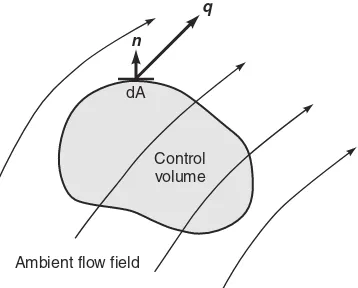
The total flux of a tracer,q, within a fluid is the sum of the advective and diffusive fluxes and is given by
q⫽qa⫹qd⫽nVc⫺D䉮(nc) (7.12)
Consider the finite control volume shown in Figure 7.8, where this control volume is con-tained within the porous medium. The law of conservation of mass requires that the net flux [M/T] of tracer mass into the control volume is equal to the rate of change of tracer mass [M/T] within the control volume. This relation is given by
ᎏ
∂ ∂ t
ᎏ
冕
Vcn dV⫹
冕
Sq·ndA ⫽
冕
VSmn dV (7.13)
whereVis the volume of the control volume,Sis the surface area of the control volume,q
is the flux vector given by Equation 7.12,nis the unit normal pointing out of the control
Control volume
Ambient flow field dA
n
q
volume, and Smis the tracer mass flux per unit volume of ground water originating within the control volume. Equation 7.13 can be simplified using the divergence theorem, which relates a surface integral to a volume integral by the relation
冕
Sq·ndA⫽冕
V䉮·qdV (7.14)
Combining Equations 7.13 and 7.14 leads to the result
ᎏ
Since the control volume is fixed in space and time, the derivative of the volume integral with respect to time is equal to the volume integral of the derivative with respect to time, and Equation 7.15 can be written in the form
冕
V冢
ᎏ∂This equation requires that the integral of the quantity in parentheses must be equal to zero for any arbitrary control volume, and this can be true only if the integrand itself is equal to zero. Following this logic, Equation 7.16 requires that
ᎏ∂
This equation can be combined with the expression for the mass flux given by Equation 7.12 and written in the expanded form
ᎏ∂
Assuming that the porosity,n, is invariant in space and time, Equation 7.18 simplifies to
ᎏ∂
In the case of incompressible fluids, conservation of fluid mass requires that
䉮·V⫽0 (7.20)
and combining Equations 7.19 and 7.20 yields the following diffusion equation:
The dispersion coefficient,D, in porous media is generally anisotropic, and denoting the principal components of the dispersion coefficient as D
i, the advection–dispersion equation
can be expressed in the form
(7.22)
where xiare the principal directions of the dispersion coefficient tensor. This form of the advection–dispersion equation, which is appropriate for flow through porous media, is identical to the form of the advection–dispersion equation used in surface waters.
Solutions to the advection–dispersion equation for specified initial and boundary con-ditions are commonly referred to as dispersion modelsorfate and transport modelsand can be either analytic or numerical. Numerical models provide discrete solutions to the advection–dispersion equation in space and time and are most useful in cases of complex geology and irregular boundary conditions. Analytic models provide continuous solutions to the advection–dispersion equation in space and time and are most useful in cases of sim-ple geology and simsim-ple boundary conditions. Most ground-water contamination problems can be analyzed assuming steady-state flow conditions, which implies that the flow veloc-ity and dispersion characteristics remain constant with time. Several useful analytic dis-persion models are described in the following sections.
7.4.1 Instantaneous Point Source
In the case where a mass,M, of conservative contaminant is injected instantaneously over a depth,H, of a uniform aquifer with mean seepage velocity,V, the resulting concentration distribution, c(x,y,t), is given by the fundamental solution to the advection–dispersion equation, which can be written in the form
(7.23)
wheretis the time since the injection of the contaminant,nis the porosity,xis the coor-dinate measured in the direction of the seepage velocity,yis the transverse (horizontal) coordinate, the contaminant source is located at the origin of the coordinate system, and DL andDTare the longitudinal and transverse dispersion coefficients. Equation 7.23 is more commonly applied in cases where a contaminant is initially mixed over a depth, H, of the aquifer, not the entire depth of the aquifer, and vertical dispersion is negligi-ble compared with longitudinal and horizontal-transverse dispersion. Contaminants are seldom released instantaneously into the ground water. However, if the duration of release is short compared to the time of interest, and if the volume spilled is small enough not to influence the ground-water flow pattern significantly near the release point, the instantaneous release assumption is justified. A contaminant mass cannot be added realistically at a point over a depth H. If the contaminant mass is added over an
areaA0and the initial concentration is c0, the following substitution into Equation 7.23
and Equation 7.23 can be applied provided that
4πt兹D苶L苶DT苶
⬎
⬎
A0 (7.25)This relation is based on the requirement that the size of the contaminated area is much greater than the size of the initial spill area.
Example 7.2 Ten kilograms of a contaminant is spilled over the top 2 m of an aquifer. The longitudinal and horizontal-transverse dispersion coefficients are 1 and 0.1 m2/day,
respectively; vertical mixing is negligible; the porosity is 0.2; and the mean seepage veloc-ity is 0.6 m/day. (a) Estimate the maximum contaminant concentrations in the ground water 1 day, 1 week, 1 month, and 1 year after the spill. (b) What is the contaminant con-centration at the spill location after 1 week?
SOLUTION From the data given,M⫽10 kg,H⫽2 m,D
L⫽1 m2/day,DT⫽0.1 m2/day,
n⫽0.2, and V⫽0.6 m/day. According to Equation 7.23, the maximum concentration,c max,
Substituting the given parameters gives
cmax(t)⫽ ⫽ ᎏ6.
which yields the results shown in Table 7.3.
(b) The concentration at the spill location (x⫽0 m,y⫽0 m) as a function of time is given by Equation 7.23 as
c(0, 0,t)⫽ ᎏ
TABLE 7.3 Results for Example 7.2
t(days) cmax(t) (mg/L)
1 6300
7 900
30 210
which at t⫽7 days gives
Hence, after 7 days, the concentration at the site of the spill is approximately 53% of the maximum concentration of 900 mg/L.
7.4.2 Continuous Point Source
In the case where a conservative contaminant of initial concentration c0is injected contin-uously at a rate Q[L3/T] into a uniform aquifer of depth Hand mean seepage velocity V,
the concentration distribution downstream of the source,c(x, y, t), is given by (Fried, 1975)
(7.26)
where the xcoordinate is in the direction of the seepage velocity; yis the transverse (horizontal) coordinate; the source is located at the origin of the coordinate system; DLand DT are the longitudinal and transverse dispersion coefficients, respectively; W (α, β) is defined as
W(α,β) is identical to the well function for a leaky aquifer that is used in ground-water hydrology. To facilitate the evaluation of Equation 7.26, values of W(α,β) are tabulated in Table 7.4. As t→ ∞, the concentration distribution given by Equation 7.26 approaches the steady-state solution (Bear, 1972)
(7.29)
whereK0is the modified Bessel function of the second kind of order zero (described in Appendix E.2).
Example 7.3 A conservative contaminant is injected continuously through a 4-m-deep perforated well into an aquifer with a mean seepage velocity of 0.8 m/day and longitudi-nal and transverse dispersion coefficients of 2 and 0.2 m2/day, respectively. If the injection
rate of the contaminated water is 0.7 m3/day, with a contaminant concentration of
100 mg/L, estimate the steady-state contaminant concentrations at locations 1, 10, 100, and 1000 m downstream of the injection well. Neglect vertical diffusion.
α β 0.00 0.002 0.004 0.007 0.01 0.02 0.04 0.06 0.08 0.10 0.00 12.6611 11.2748 10.1557 9.4425 8.0569 6.6731 5.8456 5.2950 4.8541 1⫻10⫺6 13.2383 12.4417 11.2711 10.1557
2⫻10⫺6 12.5451 12.1013 11.2259 10.1554
5⫻10⫺6 11.6289 11.4384 10.9642 10.1290 9.4425 8⫻10⫺6 11.1589 11.0377 10.7151 10.0602 9.4313
1⫻10⫺5 10.9357 10.8382 10.5725 10.0034 9.4176 8.0569 2⫻10⫺5 10.2426 10.1932 10.0522 9.7126 9.2961 8.0558
5⫻10⫺5 9.3263 9.3064 9.2480 9.0957 8.8827 8.0080 6.6730 7⫻10⫺5 8.9899 8.9756 8.9336 8.8224 8.6625 7.9456 6.6726
SOLUTION From the data given, H⫽4 m, V⫽0.8 m/day, D
L⫽2 m2/day, DT⫽
0.2 m2/day,Q⫽0.7 m3/day, and c
0⫽100 mg/L⫽0.1 kg/m3. The steady-state concentration
is given by Equation 7.29 as
c(x,y)⫽
冤
ᎏThe steady-state downstream concentrations are given listed in Table 7.5.
7.4.3 Continuous Plane Source
The case where a conservative contaminant of concentration c0is continuously released
from a plane source of dimension Y⫻Zis illustrated in Figure 7.9. The resulting concen-tration distribution,c(x,y,z,t), is given by (Domenico and Robbins, 1985)
(7.30)
whereVis the mean seepage velocity, and αx,αy, and αzare the dispersivities in the
coor-dinate directions. The dispersivity in a porous medium is defined as the dispersion coefficient divided by the mean seepage velocity, where
αx⫽ ᎏ In Equation 7.30,xis the longitudinal (flow) direction,yis the horizontal-transverse direc-tion, and zis the vertical-transverse direction. If there is no spreading in the vertical,z, direction, the error functions containing the zterms in Equation 7.30 are ignored and c0/8
c(x,y,z,t)⫽ ᎏc
TABLE 7.5 Results for Example 7.3
x(m) c(x, 0) (kg/m3) c(x, 0) (mg/L)
1 0.0094 9.4
10 0.0037 3.7
100 0.0012 1.2
becomesc0/4 (Domenico and Schwartz, 1990). The distance, x0, from the source to the location where the contaminant plume is well mixed over the aquifer thickness,H, can be estimated by (Domenico and Palciauskas, 1982)
x0⫽ ᎏ(H⫺
αz
Z)2
ᎏ (7.32)
For distances of less than x0, Equation 7.30 is applicable; for distances greater than x0, the
distance x in the denominator of the error function of the z term is replaced by x0,
prohibiting further spreading for x⬎x0. Domenico (1987) showed that for contaminants that undergo first-order decay with a decay factor λ, Equation 7.30 becomes
Z
FIGURE 7.9 Dispersion from a continuous plane source. (From Chin, David A.,Water-Resources Engineering.Copyright © 2000. Reprinted by permission of Pearson Education, Inc., Upper Saddle River, NJ.)
Example 7.4 A continuous contaminant source is 3 m wide ⫻2 m deep and contains a contaminant at a concentration of 100 mg/L. The mean seepage velocity in the aquifer is 0.4 m/day, the aquifer is 7 m deep, and the longitudinal, horizontal-transverse, and verti-cal-transverse dispersivities are 3, 0.3, and 0.03 m, respectively. (a) Assuming that the contaminant is conservative, determine the downstream location at which the nant plume will be fully mixed over the depth of the aquifer. (b) Estimate the contami-nant concentrations at the water table at locations 10, 100, and 1000 m downstream of the source after 10 years. (c) If the contaminant undergoes biodegradation with a decay rate of 0.01 day⫺1, estimate the effect on the concentrations downstream of the source.
SOLUTION (a) From the data given, Y⫽3 m, Z⫽2 m, c
0⫽100 mg/L⫽0.1 kg/m3,
V⫽0.4 m/day,H⫽7 m,α
x⫽3 m,αy⫽0.3 m, and αz⫽0.03 m. The contaminant plume
becomes well mixed at a distance x0 downstream, where x0 is given by Equation
Since the contaminant becomes well mixed at x0⫽833 m, this formulation can only be used for calculating the concentrations at xⱕ833 m. At x⫽10 m and x⫽100 m, the equa-tion yields the results shown in Table 7.6.
Atx⫽1000 m, the plume is well mixed over the vertical, and the contaminant concen-tration is calculated by replacing xbyx0(⫽833 m) in the denominator of the error func-tion in the zterm to yield
TABLE 7.6 Results for Example 7.4(b)
c(x, 0, 0, 3650) c(x, 0, 0, 3650)
x(m) (kg/m3) (mg/L)
10 0.046 46
100 0.0090 9.0
(c) If the contaminant undergoes first-order decay with λ⫽0.01 day⫺1, the
concentra-which simplifies to
c(x, 0, 0, 3650)⫽0.05 exp(⫺0.0234x) erfc
冢
ᎏx⫺The results of this example show that biodegradation will have a significant effect on the contaminant concentrations downstream of the source. Beyond x⫽100 m, the biode-graded contaminant concentrations are negligible.
7.5 TRANSPORT PROCESSES
Dispersion of contaminants in ground water is caused by spatial variations in hydraulic conductivity and, to a much smaller extent, by pore-scale mixing and molecular diffusion. Pore-scale mixing results from the differential movement of ground water through pores of various sizes and shapes, a process called mechanical dispersion; the combination of mechanical dispersion and molecular diffusion is called hydrodynamic dispersion. Dispersion caused by large-scale variations in hydraulic conductivity is called macrodis-persion. Consider a porous medium in which several samples of characteristic size Lare tested for their hydraulic conductivity,K. The hydraulic conductivity (K) is then a random
x⫺0.4(3650)[1⫹4(0.01)(3/0.4)]1/2
ᎏᎏᎏᎏ
2[3(0.4)(3650)]1/2
TABLE 7.7 Results for Example 7.4(c)
c(x, 0, 0, 3650) c(x, 0, 0, 3650)
x(m) (kg/m3) (mg/L)
10 0.015 15
space function (RSF) with support scale L. Assuming that Kis log normally distributed, it is convenient to work with the variable Ydefined as
Y⫽lnK (7.34)
whereY is a normally distributed random space function, characterized by a mean,〈Y〉; variance, σ2
Y; and correlation length scales,λi, in the xi-coordinate directions. The
geo-metric mean hydraulic conductivity,KG, is related to 〈Y〉by
KG⫽e〈Y〉 (7.35)
Freeze (1975) analyzed data from a variety of geologic cores, and the statistics of the measured hydraulic conductivities are tabulated in Table 7.8. These data indicate relatively high values of σY, which reflect a significant degree of variability about the mean hydraulic
conductivity. The variance of the hydraulic conductivity is inversely proportional to the magnitude of the support scale, with larger support scales resulting in smaller variances in the hydraulic conductivity. Consequently, whenever values of σYare cited, it is sound
prac-tice also to state the corresponding support scale. The support scale of the data shown in Table 7.8 is on the order of 10 cm. The spatial covariance of Ymust also be associated with a stated support scale, since both σYand the correlation length scale,λi, depend on the
sup-port scale. Larger supsup-port scales generally yield larger correlation length scales. Porous media in which the correlation length scales of the hydraulic conductivity in the principal directions differ from each other are called anisotropic media, and porous media where the correlation length scales of the hydraulic conductivity in the principal directions are all equal are called isotropic media. Detailed discussions of dispersion in both isotropic and anisotropic media can be found in Dagan (1989), Chin and Wang (1992), Gelhar (1993), and Chin (1997). The mean seepage velocity,Vi, in isotropic porous media is given the the Darcy equation,
(7.36)
whereKeffis the effective hydraulic conductivity,neis the effective porosity, and Jiis the
slope of the piezometric surface in the i-direction. The effective hydraulic conductivity in Vi⫽ ⫺ ᎏK
n
e
e
ff
ᎏJi TABLE 7.8 Hydraulic Conductivity Statistics
〈Y〉⫽〈lnK〉
Formation (K in m/day) KG(m/day) σY
Sandstone ⫺2.0 0.13 0.92
⫺0.98 0.38 0.46
Sand and gravel — — 1.01
— — 1.24
— — 1.66
Silty clay ⫺0.15 0.86 2.14
Loamy sand 0.59 1.81 1.98
isotropic media can be expressed in terms of the statistics of the hydraulic conductivity field by the relations (Dagan, 1989)
(7.37)
The dispersion coefficient in porous media can be stated generally as a tensor quantity, Dij, which is typically expressed in terms of the magnitude of the mean seepage velocity, V, by the relation (Bear, 1979)
Dij⫽α
ijV (7.38)
whereαijis the dispersivityof the porous medium. In general porous media,αijis a
sym-metric tensor with six independent components and can be written in the form
αij⫽
冤
冥
(7.39)whereαij⫽αji. In cases where the flow direction coincides with one of the principal
direc-tions of the hydraulic conductivity, the off-diagonal terms in the dispersivity tensor are equal to zero, and αijcan be written in the form
Two-dimensional flow: K
eff⫽KG
whereα11is generally taken as the dispersivity in the flow direction, and α22andα33are
the dispersivities in the horizontal and vertical transverse principal directions of the hydraulic conductivity. The component of the dispersivity in the direction of flow is called thelongitudinal dispersivity, and the other components of the dispersivity are called the transverse dispersivities.
The dispersivites used to describe the transport of contaminants in porous media can-not be taken as constant unless the contaminant cloud has traversed several correlation length scales of the hydraulic conductivity, or the contaminant cloud is sufficiently large to encompass several correlation length scales. If either of these conditions is violated, the dispersivity increases as the contaminant cloud moves through the porous medium, includes an expanding range of hydraulic conductivity variations and ultimately approaches a con-stant value called the asymptotic macrodispersivity or simply the macrodispersivity. In isotropic media, the correlation length scale,λ, of the hydraulic conductivity is the same in all directions, and the components of the macrodispersivity can be estimated using the approximate relations (Dagan, 1989; Chin and Wang, 1992)
where it is interesting to note that the heterogeneous structure of the porous medium does not create transverse macrodispersion. Derivation of Equation 7.41 assumes that the local-mean seepage velocity is statistically homogeneous, and the spatial correlation of the hydraulic conductivity can be represented by an exponential function of spatial separation. According to Chin and Wang (1992), assumptions in the theoretical approximations used in deriving Equation 7.41 can be taken as valid up to σY⫽1.5.
In cases where the porous medium is stratified, isotropic in the horizontal plane, and anisotropic in the vertical plane, the correlation length scale of the hydraulic conductivity in the horizontal plane can be denoted by λh, and the correlation length scale in the
verti-cal direction denoted by λv. The anisotropy ratio,e, is then defined by
e⫽ ᎏ
λ λ
h v
ᎏ (7.42)
and is typically on the order of 0.1 in most stratified media. Gelhar and Axness (1983) have derived approximate relations to estimate the components of the macrodispersivity in the case that the flow is in the plane of isotropy. In this case, the longitudinal and trans-verse components of the macrodispersivity tensor can be estimated by
(7.43)
The relationships given in Equation 7.43 are approximately valid for σY⬍1, but the
exact range of validity has not been established (Chin, 1997). Typical values of σY,λh, and
λvin several formations are listed in Table 7.9. It is important to note that even though the
hydraulic-conductivity statistics given in Table 7.9 depend on the support scale of the sam-ples used to derive the statistics, the macrodispersivities calculated using these statistics are (theoretically) independent of the support scale of the samples. In estimating the (total) dispersivity in porous media, the macrodispersivities calculated using either Equation 7.41
α11⫽σY2λh, α22⫽α33⫽0
TABLE 7.9 Variances and Correlation Length Scales of Hydraulic Conductivity
Formation σY λh(m) λv(m) Reference
Sandstone 1.5–2.2 — 0.3–1.0 Bakr (1976)
0.4 8 3 Goggin et al. (1988)
Sand 0.9 ⬎3 0.1 Byers and Stephens (1983)
0.6 3 0.12 Sudicky (1986)
0.5 5 0.26 Hess (1989)
0.4 8 0.34 Woodbury and Sudicky
(1991)
0.4 4 0.2 Robin et al. (1991)
0.2 5 0.21 Woodbury and Sudicky
(1991)
Sand and 5 12 1.5 Boggs et al. (1990)
gravel 2.1 13 1.5 Rehfeldt et al. (1989)
1.9 20 0.5 Hufschmied (1986)
or 7.43 are additive to the dispersivities associated with hydrodynamic dispersion, which result from pore-scale mixing and molecular diffusion.
Example 7.5 Several hydraulic conductivity measurements in an isotropic aquifer indi-cate that the spatial covariance,CY, of the log-hydraulic conductivity can be approximated by the equation
r3is measured in the vertical plane. The mean hydraulic gradient is 0.001, the effective porosity is 0.2, and the mean log-hydraulic conductivity is 2.5 (where the hydraulic con-ductivity is in m/day). Estimate the effective hydraulic conductivity and the macrodisper-sion coefficient in the aquifer.
SOLUTION From the data given, the hydraulic conductivity field is described statisti-cally by 〈Y〉⫽2.5,σ
Y⫽0.5, and λ⫽5 m. The geometric mean hydraulic conductivity,KG,
is given by Equation 7.35 as
KG⫽e〈Y〉⫽e2.5⫽12 m/day
and the effective hydraulic conductivity, for three-dimensional flow, is given by Equation 7.37 as
The mean seepage velocity,V, in the aquifer is given by Equation 7.36 as
V⫽ ⫺ ᎏK
Since σY⫽0.5 and λ⫽5 m, the longitudinal macrodispersivity, α11, can be estimated by Equation 7.41 as
α11⫽σY2λ⫽(0.5)2(5)⫽1.25 m
and, according to Equation 7.41, the theoretical transverse macrodispersivities are both zero. The longitudinal dispersion coefficient,D11, is given by
D11⫽α
The relative importance of advective transport to dispersive transport can be measured by the Peclet number, Pe, defined as
(7.44)
whereVis the mean seepage velocity, Lis the characteristic length scale, and DLis the characteristic longitudinal dispersion coefficient. For Pe⬎10 advection dominates, for Pe⬍0.1 dispersion dominates, and for 0.1ⱕPeⱕ10 both advection and dispersion are important. In municipal well fields, values of Pe within several meters of the well tend to be high, indicating that contaminant transport is advection-dominated and dispersion effects are relatively small. A Peclet number, Pe
m, can be defined based on the molecular
where d is the characteristic pore size and Dm is the molecular diffusion coefficient. Previous investigations have shown that the pore-scale longitudinal dispersion coefficient is much greater than the molecular diffusion coefficient when Pe
m⬎10, and the pore-scale
transverse dispersion coefficient is much greater than the molecular diffusion coefficient when Pem⬎100 (Perkins and Johnson, 1963).
Example 7.6 The mean seepage velocity in an aquifer is 1 m/day, the mean pore size is 1 mm, and the molecular diffusion coefficient of a certain toxic contaminant in water is 10⫺9m2/s . Determine whether molecular diffusion should be considered in a pore-scale
contaminant transport model.
Since Pem⬎10, molecular diffusion has a negligible contribution to longitudinal dispersion, but since Pem⬍100, molecular diffusion will contribute significantly to transverse dispersion.
In most practical cases longitudinal dispersion is dominated by macrodispersion, hori-zontal-transverse dispersion is influenced significantly by temporal variations in the seep-age velocity, and vertical-transverse dispersion is dominated by small-scale hydrodynamic dispersion (Rehfeldt and Gelhar, 1992). Field studies indicate that horizontal-transverse dispersivities can be related to longitudinal dispersivities using a ratio of longitudinal to horizontal-transverse dispersivity in the range 6 to 20 (Anderson, 1979; Klotz et al., 1980). The horizontal-transverse dispersivity is usually much larger than the vertical-transverse dispersivity. Common practice is to estimate the longitudinal dispersivity using a theoret-ical or empirtheoret-ical relation such as Equation 7.41, estimate the horizontal-transverse disper-sivity as one-tenth of the longitudinal disperdisper-sivity, and estimate the vertical-transverse
Pe⫽ ᎏV
D L
dispersivity as one-hundredth of the longitudinal dispersivity (Zheng and Bennett, 1995). These estimates are conservative relative to those suggested by the U.S. Environmental Protection Agency (1985a), where the horizontal-transverse dispersivity is one-third of the longitudinal dispersivity and the vertical-transverse dispersivity is one-twentieth of the longitudinal dispersivity.
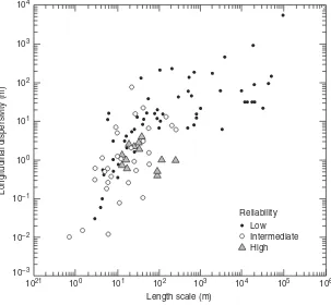
Longitudinal dispersivities derived from 59 sites around the world have been collated by Gelhar and colleagues (1992) and are shown in Figure 7.10. Data from these sites yielded 106 values of longitudinal dispersivity, ranging from 0.01 to 5500 m at scales of 0.75 m to 100 km. Based on the results shown in Figure 7.10, it is clear that the longitudi-nal dispersivity increases with the distance traveled by the contaminant cloud (i.e., scale), indicating that field formations are seldom homogeneous and that the variability in hydraulic conductivity increases with scale. Of all the experiments reviewed by Gelhar and colleagues (1992), only 14 studies were considered to provide highly reliable estimates of the dispersivity, a further 31 values were considered of intermediate reliability, and the most reliable dispersivity estimates were at the lower end of the length scale. In the absence of field measurements of the hydraulic conductivity, from which the spatial sta-tistics are parameterized by 〈Y〉,σY, and λ, Figure 7.10 provides a useful basis for
esti-mating the dispersivity in porous formations. The length scale, L, in Figure 7.10 can be taken as either the distance travelled by a tracer released from a point or the length scale measuring the size of the tracer cloud. In either case, the length scale, L, measures the spa-tial extent of seepage velocity variations experienced by the tracer cloud. Analyses by
Length scale (m)
Longitudinal dispersivity (m)
104
1021
10–3
10–2 10–1
106
100
101
102
103
105
104
High Intermediate Low Reliability
103
102
101
100
Neuman (1990) indicate that the longitudinal macrodispersivity,α11, can be related to the
travel distance,L, by the relation
(7.46)
whereα11andLare both measured in meters. For L⬍100 m, a better match with field data
was obtained using
(7.47)
Analyses by Al-Suwaiyan (1998) demonstrate that the observed macrodispersivities reported by Gelhar and colleagues (1992) are scattered about the mean (approximated by Equations 7.46 and 7.47), with the upper limit of the scatter at about five times the mean and the lower limit at about one-fifth of the mean. These uncertainty limits should be accounted for whenever Equations 7.46 and 7.47 are used in contaminant-transport pre-dictions. For very small scales, on the order of the pore size, dispersion is caused prima-rily by pore-scale mechanical dispersion and molecular diffusion, where the longitudinal and transverse dispersivities can be estimated by the relations
(7.48)
whereαL* and αT* are pore-scale longitudinal and transverse dispersivities respectively,Dm
is the molecular diffusion coefficient in water,τis the tortuosity (which accounts for the effect of the solid matrix on diffusion), and Vis the mean seepage velocity. The molecular diffusion coefficient divided by the tortuosity represents the effective molecular diffusion coefficient in porous media and is sometimes called the bulk diffusion coefficient. Values ofαL* are typically on the order of the pore size of the porous medium,αT* is typically on
the order of 0.1 to 0.01αL* (Delleur, 1998),τis typically in the range 2 to 100 (lower
val-ues are associated with coarse material such as sands; higher valval-ues are associated with finer material such as clays), and typical values of the molecular diffusion coefficient are in the range 10⫺5to 10⫺3m2/day at 25⬚C (Fetter, 1999).
For travel distances longer than 3500 m, the longitudinal dispersivity tends to asymp-tote to an upper limit that is consistent with a finite variability in the hydraulic conductiv-ity. In cases where the dispersivity increases with travel distance, the Fickian assumption of a constant dispersion coefficient is not supported and the dispersion is termed non-Fickian. However, a Fickian approximation to the mixing process is obtained by adjusting the dispersion coefficient with length scale, and the advection–dispersion equation can be used to approximate the dispersion process. Typical values of the longitutinal dispersivity for various ranges of length scales are shown in Table 7.10.
Example 7.7 A contaminant plume in an aquifer is approximately 50 m long, 10 m wide, and 3 m deep. The characteristic pore size in the aquifer is 3 mm, the molecular diffusion
αL⫽αL*⫹ ᎏ
D τV
m ᎏ
αT⫽αT*⫹ ᎏ
D τV
m ᎏ
α11⫽0.0169L1.53, L⬍100 m
coefficient is 2⫻10⫺9m2/s, the tortuosity is 1.5, and the mean seepage velocity is
0.5 m/day. Estimate the components of the dispersion coefficient.
SOLUTION From the data given,Lx⫽50 m,Ly⫽10 m,Lz⫽3 m,Dm⫽2⫻10⫺9m2/s⫽
1.73⫻10⫺4m2/day,τ⫽1.5, and V⫽0.5 m/day. The length scale, L, of the contaminant
plume can be approximated by the relation
L⫽兹L苶x苶Ly苶⫽兹5苶0苶(1苶0苶)苶⫽22 m
and since L⬍100 m, the longitudinal macrodispersivity can be estimated by Equa-tion 7.47 as
α11⫽0.0169L1.53⫽0.0169(22)1.53⫽1.9 m
The horizontal-transverse macrodispersivity, α22, can be estimated as 0.1α11, which
gives
α22⫽0.1α11⫽0.1(1.9)⫽0.19 m
and the vertical-transverse macrodispersivity,α33, can be estimated as 0.01α11, which gives
α33⫽0.01α11⫽0.01(1.9)⫽0.019 m
The local longitudinal dispersivity,αL, is given by Equation 7.48, where αL* is on the order
of the pore size (0.003 m), and hence
αL⫽αL*⫹ ᎏ
The principal components of the dispersion coefficient are then given by
D11⫽(α
11⫹αL)V⫽(1.9⫹0.0032)(0.5)⫽0.95 m2/day
D22⫽(α
22⫹αT)V⫽(0.19⫹0.00053)(0.5)⫽0.095 m2/day
D33⫽(α
33⫹αT)V⫽(0.019⫹0.00053)(0.5)⫽0.0097 m2/day
It must be emphasized that these estimates of the dispersion coefficient are order-of-mag-nitude estimates only, and it would be entirely appropriate to take D11⫽1 m2/day,
D22⫽0.1 m2/day, and D
33⫽0.01 m2/day. The dominance of macrodispersion over
pore-scale mechanical dispersion and molecular diffusion in the longitudinal and horizontal-transverse directions are evident.
Field experiments to estimate local values of dispersivity at a particular site typically consist of releasing dye from an injection well, measuring the breakthrough dye con-centrations at a downstream well, and estimating the dispersivity based on the rate of growth of variance of the dye cloud or matching the measured concentrations to a solu-tion to the advecsolu-tion–dispersion equasolu-tion. These tests can be either natural-gradient tests orforced-gradient tests. Natural-gradient tests are conducted under natural flow conditions, and forced-gradient tests are conducted under artificial (pumping) stress con-ditions. Examples of forced-gradient conditions include converging radial flow, and flows induced by placing an injection well upstream of a pumping well. It is important to keep in mind that the dispersivities estimated under different stress conditions tend to be different. Results reported by Tiedeman and Hsieh (2004) show that among forced-gra-dient tests, a converging radial-flow test tends to yield the smallest longitudinal dispersiv-ity (α11), an equal-strength two-well test tends to yield the largest α11, and an unequal
strength two-well test tends to yield an intermediate value of α11. Tiedeman and Hsieh
(2004) also showed that values of α11 estimated under forced-gradient conditions can
significantly underestimate α
11under natural-gradient flow conditions. In support of this
result, Chao et al. (2000) reported that based on numerical simulations using point sources, α11from radial-flow tests were 5 to 10 times smaller than α11for natural-gradient tests.
7.6 FATE PROCESSES
7.6.1 Sorption
Models that describe the partitioning of dissolved mass onto solid surfaces are called sorp-tion isotherms, since they describe sorption at a constant temperature. The most widely used sorption isotherm is the Freundlich isotherm, given by
F⫽K
Fcnaq (7.49)
whereFis the mass of tracer sorbed per unit mass of solid phase,caqis the concentration
of the tracer dissolved in the water (aqueous concentration), and KFandnare constants. The constant,n, is typically in the range 0.7 to 1.2 (Domenico and Schwartz, 1998), and for many contaminants at low concentrations, the constant n is approximately equal to unity. In this case, the Freundlich isotherm, Equation 7.49, is linear and is written in the form
F⫽K
dcaq (7.50)
where Kdis called the distribution coefficient [L3/M] and is defined as the ratio of the
sorbed tracer mass per unit mass of solid matrix to the aqueous concentration. Although the Freundlich isotherm is widely used in practice, it has an important limitation in that it places no limit on the sorption capacity of the solid matrix. The Langmuir isothermallows for a maximum sorption capacity on the solid matrix and is defined by
F⫽ ᎏ 1
K
⫹ lS苶
K c
l a
c
q
aq
ᎏ (7.51)
whereKlis the Langmuir constantandS苶is the maximum sorption capacity. At low solute concentrations, when Klcaq⬍⬍1, the Langmuir isotherm is similar to the linear Freundlich isotherm, with Flinearly proportional to caq, while at high concentrations, when Klcaq⬎⬎1,
F approaches the limiting value of S苶. Despite the apparent advantages of using the Langmuir isotherm, the linear Freundlich isotherm remains the most widely used.
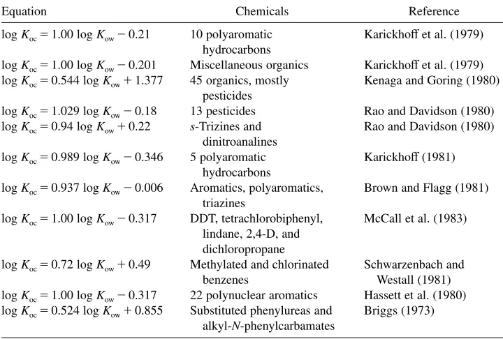
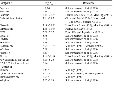
In applying linear isotherms such as Equation 7.50, care should be taken since the actual isotherm is usually piecewise linear, and therefore extrapolation beyond the range of experimental conditions used to estimate Kdis not recommended (Fetter, 1992). Values ofKdin Equation 7.50 range from near zero to 103cm3/g or greater. In the case of organic
compounds, the mass of the organic compound sorbed per unit mass of solid matrix has been observed to depend primarily on the amount of organic carbon in the solid matrix (Karickhoffet al., 1979), and it is more appropriate to deal with the organic carbon sorp-tion coefficient Koc, which is defined as the ratio of sorbed mass of organic compound per
unit mass of organic carbon to the aqueous concentration. Therefore, the distribution coefficient,Kd, is related to the organic carbon sorption coefficient,Koc, by
Kd⫽focKoc (7.52)