1. 1. A Gentle Introduction to Spark
1. What is Apache Spark?
1. Spark Applications
3. Using Spark from Scala, Java, SQL, Python, or R
1. Key Concepts
4. Starting Spark
5. SparkSession
6. DataFrames
1. Partitions
7. Transformations
1. Lazy Evaluation
8. Actions
9. Spark UI
10. A Basic Transformation Data Flow
11. DataFrames and SQL
2. 2. Structured API Overview
1. Spark’s Structured APIs
2. DataFrames and Datasets
3. Schemas
4. Overview of Structured Spark Types
1. Columns
2. Rows
3. Spark Value Types
4. Encoders
5. Overview of Spark Execution
1. Logical Planning
2. Physical Planning
3. Execution
3. 3. Basic Structured Operations
1. Chapter Overview
2. Schemas
3. Columns and Expressions
1. Columns
2. Expressions
4. Records and Rows
1. Creating Rows
5. DataFrame Transformations
1. Creating DataFrames
3. Converting to Spark Types (Literals)
4. Adding Columns
5. Renaming Columns
6. Reserved Characters and Keywords in Column Names
7. Removing Columns
8. Changing a Column’s Type (cast)
9. Filtering Rows
10. Getting Unique Rows
11. Random Samples
12. Random Splits
13. Concatenating and Appending Rows to a DataFrame
14. Sorting Rows
15. Limit
16. Repartition and Coalesce
17. Collecting Rows to the Driver
4. 4. Working with Different Types of Data
1. Chapter Overview
1. Where to Look for APIs
2. Working with Booleans
3. Working with Numbers
4. Working with Strings
1. Regular Expressions
5. Working with Dates and Timestamps
6. Working with Nulls in Data
1. Drop
2. Fill
3. Replace
7. Working with Complex Types
1. Structs
2. Arrays
3. split
4. Array Contains
5. Explode
6. Maps
8. Working with JSON
9. User-Defined Functions
1. What are aggregations?
2. Aggregation Functions
1. count
2. Count Distinct
3. Approximate Count Distinct
4. First and Last
5. Min and Max
6. Sum
7. sumDistinct
8. Average
9. Variance and Standard Deviation
10. Skewness and Kurtosis
11. Covariance and Correlation
12. Aggregating to Complex Types
3. Grouping
1. Grouping with expressions
2. Grouping with Maps
4. Window Functions
1. Rollups
2. Cube
3. Pivot
5. User-Defined Aggregation Functions
6. 6. Joins
1. What is a join?
1. Join Expressions
2. Join Types
2. Inner Joins
3. Outer Joins
4. Left Outer Joins
5. Right Outer Joins
6. Left Semi Joins
7. Left Anti Joins
8. Cross (Cartesian) Joins
9. Challenges with Joins
1. Joins on Complex Types
2. Handling Duplicate Column Names
1. Node-to-Node Communication Strategies
7. 7. Data Sources
1. The Data Source APIs
1. Basics of Reading Data
2. Basics of Writing Data
3. Options
2. CSV Files
1. CSV Options
2. Reading CSV Files
3. Writing CSV Files
3. JSON Files
1. JSON Options
2. Reading JSON Files
3. Writing JSON Files
4. Parquet Files
1. Reading Parquet Files
2. Writing Parquet Files
5. ORC Files
1. Reading Orc Files
2. Writing Orc Files
6. SQL Databases
1. Reading from SQL Databases
2. Query Pushdown
3. Writing to SQL Databases
7. Text Files
1. Reading Text Files
2. Writing Out Text Files
8. Advanced IO Concepts
1. Reading Data in Parallel
2. Writing Data in Parallel
3. Writing Complex Types
8. 8. Spark SQL
1. Spark SQL Concepts
1. What is SQL?
2. Big Data and SQL: Hive
3. Big Data and SQL: Spark SQL
1. SparkSQL Thrift JDBC/ODBC Server
2. Spark SQL CLI
3. Spark’s Programmatic SQL Interface
3. Tables
1. Creating Tables
2. Inserting Into Tables
3. Describing Table Metadata
4. Refreshing Table Metadata
5. Dropping Tables
4. Views
1. Creating Views
2. Dropping Views
5. Databases
1. Creating Databases
2. Setting The Database
3. Dropping Databases
6. Select Statements
1. Case When Then Statements
7. Advanced Topics
1. Complex Types
2. Functions
3. Spark Managed Tables
4. Subqueries
5. Correlated Predicated Subqueries
8. Conclusion
9. 9. Datasets
1. What are Datasets?
1. Encoders
2. Creating Datasets
1. Case Classes
3. Actions
4. Transformations
1. Filtering
2. Mapping
5. Joins
6. Grouping and Aggregations
10. 10. Low Level API Overview
1. The Low Level APIs
1. When to use the low level APIs?
2. The SparkConf
3. The SparkContext
4. Resilient Distributed Datasets
5. Broadcast Variables
6. Accumulators
11. 11. Basic RDD Operations
1. RDD Overview
1. Python vs Scala/Java
2. Creating RDDs
1. From a Collection
2. From Data Sources
3. Manipulating RDDs
4. Transformations
1. Distinct
2. Filter
3. Map
4. Sorting
5. Random Splits
5. Actions
6. Saving Files
1. saveAsTextFile
2. SequenceFiles
3. Hadoop Files
7. Caching
8. Interoperating between DataFrames, Datasets, and RDDs
9. When to use RDDs?
1. Performance Considerations: Scala vs Python
2. RDD of Case Class VS Dataset
1. Advanced “Single RDD” Operations
1. Pipe RDDs to System Commands
2. mapPartitions
3. foreachPartition
4. glom
2. Key Value Basics (Key-Value RDDs)
1. keyBy
2. Mapping over Values
3. Extracting Keys and Values
4. Lookup
3. Aggregations
1. countByKey
2. Understanding Aggregation Implementations
3. aggregate
6. Controlling Partitions
1. coalesce
7. repartitionAndSortWithinPartitions
1. Custom Partitioning
8. repartitionAndSortWithinPartitions
9. Serialization
13. 13. Distributed Variables
1. Chapter Overview
2. Broadcast Variables
3. Accumulators
1. Basic Example
2. Custom Accumulators
14. 14. Advanced Analytics and Machine Learning
1. The Advanced Analytics Workflow
1. Supervised Learning
2. Recommendation
3. Unsupervised Learning
4. Graph Analysis
3. Spark’s Packages for Advanced Analytics
1. What is MLlib?
4. High Level MLlib Concepts
5. MLlib in Action
1. Transformers
2. Estimators
3. Pipelining our Workflow
4. Evaluators
5. Persisting and Applying Models
6. Deployment Patterns
15. 15. Preprocessing and Feature Engineering
1. Formatting your models according to your use case
2. Properties of Transformers
3. Different Transformer Types
4. High Level Transformers
1. RFormula
2. SQLTransformers
3. VectorAssembler
5. Text Data Transformers
1. Tokenizing Text
2. Removing Common Words
3. Creating Word Combinations
4. Converting Words into Numbers
6. Working with Continuous Features
1. Bucketing
2. Scaling and Normalization
3. StandardScaler
7. Working with Categorical Features
1. StringIndexer
2. Converting Indexed Values Back to Text
3. Indexing in Vectors
4. One Hot Encoding
1. PCA
2. Interaction
3. PolynomialExpansion
9. Feature Selection
1. ChisqSelector
10. Persisting Transformers
11. Writing a Custom Transformer
16. 16. Preprocessing
1. Formatting your models according to your use case
2. Properties of Transformers
3. Different Transformer Types
4. High Level Transformers
1. RFormula
2. SQLTransformers
3. VectorAssembler
5. Text Data Transformers
1. Tokenizing Text
2. Removing Common Words
3. Creating Word Combinations
4. Converting Words into Numbers
6. Working with Continuous Features
1. Bucketing
2. Scaling and Normalization
3. StandardScaler
7. Working with Categorical Features
1. StringIndexer
2. Converting Indexed Values Back to Text
3. Indexing in Vectors
4. One Hot Encoding
8. Feature Generation
1. PCA
2. Interaction
3. PolynomialExpansion
9. Feature Selection
1. ChisqSelector
10. Persisting Transformers
17. 17. Classification
1. Logistic Regression
1. Model Hyperparameters
2. Training Parameters
3. Prediction Parameters
4. Example
5. Model Summary
2. Decision Trees
1. Model Hyperparameters
2. Training Parameters
3. Prediction Parameters
4. Example
3. Random Forest and Gradient Boosted Trees
1. Model Hyperparameters
2. Training Parameters
3. Prediction Parameters
4. Example
4. Multilayer Perceptrons
1. Model Hyperparameters
2. Training Parameters
3. Example
5. Naive Bayes
1. Model Hyperparameters
2. Training Parameters
3. Prediction Parameters
4. Example.
6. Evaluators
7. Metrics
18. 18. Regression
1. Linear Regression
1. Example
2. Training Summary
2. Generalized Linear Regression
1. Model Hyperparameters
2. Training Parameters
3. Prediction Parameters
5. Training Summary
3. Decision Trees
4. Random Forest and Gradient-boosted Trees
5. Survival Regression
1. Model Hyperparameters
2. Training Parameters
3. Prediction Parameters
4. Example
6. Isotonic Regression
7. Evaluators
8. Metrics
19. 19. Recommendation
1. Alternating Least Squares
1. Model Hyperparameters
2. Training Parameters
2. Evaluators
3. Metrics
1. Regression Metrics
2. Ranking Metrics
20. 20. Clustering
1. K-means
1. Model Hyperparameters
2. Training Parameters
3. K-means Summary
2. Bisecting K-means
1. Model Hyperparameters
2. Training Parameters
3. Bisecting K-means Summary
3. Latent Dirichlet Allocation
1. Model Hyperparameters
2. Training Parameters
3. Prediction Parameters
4. Gaussian Mixture Models
1. Model Hyperparameters
2. Training Parameters
3. Gaussian Mixture Model Summary
1. Building A Graph
2. Querying the Graph
1. Subgraphs
3. Graph Algorithms
1. PageRank
2. In and Out Degrees
3. Breadth-first Search
4. Connected Components
5. Motif Finding
6. Advanced Tasks
22. 22. Deep Learning
1. Ways of using Deep Learning in Spark
2. Deep Learning Projects on Spark
Spark: The Definitive Guide
by Matei Zaharia and Bill ChambersCopyright © 2017 Databricks. All rights reserved. Printed in the United States of America.
Published by O’Reilly Media, Inc. , 1005 Gravenstein Highway North, Sebastopol, CA 95472.
O’Reilly books may be purchased for educational, business, or sales promotional use. Online editions are also available for most titles (
http://oreilly.com/safari ). For more information, contact our corporate/institutional sales department: 800-998-9938 or [email protected] .
Editor: Ann Spencer
Production Editor: FILL IN PRODUCTION EDITOR Copyeditor: FILL IN COPYEDITOR
Proofreader: FILL IN PROOFREADER Indexer: FILL IN INDEXER
Interior Designer: David Futato Cover Designer: Karen Montgomery Illustrator: Rebecca Demarest
Revision History for the First
Edition
2017-01-24: First Early Release 2017-03-01: Second Early Release 2017-04-27: Third Early Release
See http://oreilly.com/catalog/errata.csp?isbn=9781491912157 for release details.
The O’Reilly logo is a registered trademark of O’Reilly Media, Inc. Spark: The Definitive Guide, the cover image, and related trade dress are trademarks of O’Reilly Media, Inc.
While the publisher and the author(s) have used good faith efforts to ensure that the information and instructions contained in this work are accurate, the
publisher and the author(s) disclaim all responsibility for errors or omissions, including without limitation responsibility for damages resulting from the use of or reliance on this work. Use of the information and instructions contained in this work is at your own risk. If any code samples or other technology this work contains or describes is subject to open source licenses or the
intellectual property rights of others, it is your responsibility to ensure that your use thereof complies with such licenses and/or rights.
Spark: The Definitive Guide
Big data processing made simpleWhat is Apache Spark?
Apache Spark is a processing system that makes working with big data simple. It is a group of much more than a programming paradigm but an ecosystem of a variety of packages, libraries, and systems built on top of the Core of Spark. Spark Core consists of two APIs. The Unstructured and Structured APIs. The Unstructured API is Spark’s lower level set of APIs including Resilient Distributed Datasets (RDDs), Accumulators, and Broadcast variables. The Structured API consists of DataFrames, Datasets, Spark SQL and is the
interface that most users should use. The difference between the two is that one is optimized to work with structured data in a spreadsheet-like interface while the other is meant for manipulation of raw java objects. Outside of Spark Core sit a variety of tools, libraries, and languages like MLlib for performing
machine learning, the GraphX module for performing graph processing, and SparkR for working with Spark clusters from the R langauge.
Spark’s Basic Architecture
Typically when you think of a “computer” you think about one machine sitting on your desk at home or at work. This machine works perfectly well for watching movies, or working with spreadsheet software but as many users likely experienced at some point, there are somethings that your computer is not powerful enough to perform. One particularly challenging area is data processing. Single machines simply cannot have enough power and resources to perform computations on huge amounts of information (or the user may not have time to wait for the computation to finish). A cluster, or group of
machines, pools the resources of many machines together. Now a group of machines alone is not powerful, you need a framework to coordinate work across them. Spark is a tool for just that, managing and coordinating the resources of a cluster of computers.
Spark Applications
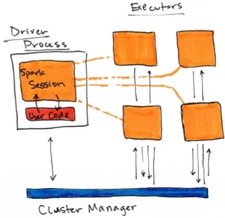
Spark Applications consist of a driver process and a set of executor
processes. The driver process, Figure 1-2, sits on the driver node and is responsible for three things: maintaining information about the Spark
application, responding to a user’s program, and analyzing, distributing, and scheduling work across the executors. As suggested by figure 1-1, the driver process is absolutely essential - it’s the heart of a Spark Application and maintains all relevant information during the lifetime of the application.
An executor is responsible for two things: executing code assigned to it by the driver and reporting the state of the computation back to the driver node.
The last piece relevant piece for us is the cluster manager. The cluster manager controls physical machines and allocates resources to Spark applications. This can be one of several core cluster managers: Spark’s standalone cluster
Figure 1-1 shows, on the left, our driver and on the right the four worker nodes on the right.
NOTE:
Spark, in addition to its cluster mode, also has a local mode. Remember how the driver and executors are processes? This means that Spark does not dictate where these processes live. In local mode, these processes run on your
Using Spark from Scala, Java, SQL,
Python, or R
As you likely noticed in the previous figures, Spark works with multiple languages. These language APIs allow you to run Spark code from another language. When using the Structured APIs, code written in any of Spark’s supported languages should perform the same, there are some caveats to this but in general this is the case. Before diving into the details, let’s just touch a bit on each of these langauges and their integration with Spark.
Scala
Spark is primarily written in Scala, making it Spark’s “default” language. This book will include examples of Scala where ever there are code samples. Python
Python supports nearly everything that Scala supports. This book will include Python API examples wherever possible.
Java
Even though Spark is written in Scala, Spark’s authors have been careful to ensure that you can write Spark code in Java. This book will focus primarily on Scala but will provide Java examples where relevant.
SQL
Spark supports user code written in ANSI 2003 Compliant SQL. This makes it easy for analysts and non-programmers to leverage the big data powers of Spark. This book will include numerous SQL examples.
R
Key Concepts
Now we have not exhaustively explored every detail about Spark’s
architecture because at this point it’s not necessary to get us closer to running our own Spark code. The key points are that:
Spark has some cluster manager that maintains an understanding of the resources available.
The driver process is responsible for executing our driver program’s commands accross the executors in order to complete our task.
Starting Spark
SparkSession
From the beginning of this chapter we know that we leverage a driver process to maintain our Spark Application. This driver process manifests itself to the user as something called the SparkSession. The SparkSession instance is the entrance point to executing code in Spark, in any language, and is the user-facing part of a Spark Application. In Scala and Python the variable is available as spark when you start up the Spark console. Let’s go ahead and look at the SparkSession in both Scala and/or Python.
%scala spark %python spark
In Scala, you should see something like:
res0: org.apache.spark.sql.SparkSession = org.apache.spark.sql.SparkSession@27159a24 In Python you’ll see something like:
<pyspark.sql.session.SparkSession at 0x7efda4c1ccd0>
Now you need to understand how to submit commands to the SparkSession. Let’s do that by performing one of the simplest tasks that we can - creating a range of numbers. This range of numbers is just like a named column in a spreadsheet.
%scala
val myRange = spark.range(1000).toDF("number") %python
You just ran your first Spark code! We created a DataFrame with one column containing 1000 rows with values from 0 to 999. This range of number
DataFrames
A DataFrame is a table of data with rows and columns. We call the list of columns and their types a schema. A simple analogy would be a spreadsheet with named columns. The fundamental difference is that while a spreadsheet sits on one computer in one specific location, a Spark DataFrame can span potentially thousands of computers. The reason for putting the data on more than one computer should be intuitive: either the data is too large to fit on one machine or it would simply take too long to perform that computation on one machine.
The DataFrame concept is not unique to Spark. The R Language has a similar concept as do certain libraries in the Python programming language. However, Python/R DataFrames (with some exceptions) exist on one machine rather than multiple machines. This limits what you can do with a given DataFrame in python and R to the resources that exist on that specific machine. However, since Spark has language interfaces for both Python and R, it’s quite easy to convert to Pandas (Python) DataFrames to Spark DataFrames and R
DataFrames to Spark DataFrames (in R).
Note
Partitions
In order to leverage the the resources of the machines in cluster, Spark breaks up the data into chunks, called partitions. A partition is a collection of rows that sit on one physical machine in our cluster. A DataFrame consists of zero or more partitions.
When we perform some computation, Spark will operate on each partition in parallel unless an operation calls for a shuffle, where multiple partitions need to share data. Think about it this way, if you need to run some errands you typically have to do those one by one, or serially. What if you could instead give one errand to a worker who would then complete that task and then report back to you? In that scenario, the key is to break up errands efficiently so that you can get as much work done in as little time as possible. In the Spark world an “errand” is equivalent to computation + data and a “worker” is equivalent to an executor.
Transformations
In Spark, the core data structures are immutable meaning they cannot be changed once created. This might seem like a strange concept at first, if you cannot change it, how are you supposed to use it? In order to “change” a DataFrame you will have to instruct Spark how you would like to modify the DataFrame you have into the one that you want. These instructions are called
transformations. Transformations are how you, as user, specify how you would like to transform the DataFrame you currently have to the DataFrame that you want to have. Let’s show an example. To computer whether or not a number is divisible by two, we use the modulo operation to see the remainder left over from dividing one number by another.
We can use this operation to perform a transformation from our current
DataFrame to a DataFrame that only contains numbers divisible by two. To do this, we perform the modulo operation on each row in the data and filter out the results that do not result in zero. We can specify this filter using a where
clause.
%scala
val divisBy2 = myRange.where("number % 2 = 0") %python
divisBy2 = myRange.where("number % 2 = 0")
Note
Now if you worked with any relational databases in the past, this should feel quite familiar. You might say, aha! I know the exact expression I should use if this was a table.
SELECT * FROM myRange WHERE number % 2 = 0
DataFrame into a table.
Lazy Evaluation
Actions
To trigger the computation, we run an action. An action instructs Spark to compute a result from a series of transformations. The simplest action is count which gives us the total number of records in the DataFrame.
%scala
divisBy2.count() %python
divisBy2.count()
Spark UI
During Spark’s execution of the previous code block, users can monitor the progress of their job through the Spark UI. The Spark UI is available on port 4040 of the driver node. If you are running in local mode this will just be the http://localhost:4040. The Spark UI maintains information on the state of our Spark jobs, environment, and cluster state. It’s very useful, especially for tuning and debugging. In this case, we can see one Spark job with one stage and nine tasks were executed.
A Basic Transformation Data Flow
In the previous example, we created a DataFrame from a range of data.Interesting, but not exactly applicable to industry problems. Let’s create some DataFrames with real data in order to better understand how they work. We’ll be using some flight data from the United States Bureau of Transportation statistics.
We touched briefly on the SparkSession as the interface the entry point to
performing work on the Spark cluster. the SparkSession can do much more than simply parallelize an array it can create DataFrames directly from a file or set of files. In this case, we will create our DataFrames from a JavaScript Object Notation (JSON) file that contains some summary flight information as
collected by the United States Bureau of Transport Statistics. In the folder provided, you’ll see that we have one file per year.
%fs ls /mnt/defg/chapter-1-data/json/
This file has one JSON object per line and is typically refered to as line-delimited JSON.
%fs head /mnt/defg/chapter-1-data/json/2015-summary.json
What we’ll do is start with one specific year and then work up to a larger set of data. Let’s go ahead and create a DataFrame from 2015. To do this we will use the DataFrameReader (via spark.read) interface, specify the format and the path.
%scala
val flightData2015 = spark .read
.json("/mnt/defg/chapter-1-data/json/2015-summary.json") %python
.json("/mnt/defg/chapter-1-data/json/2015-summary.json") flightData2015
You’ll see that our two DataFrames (in Scala and Python) each have a set of columns with an unspecified number of rows. Let’s take a peek at the data with a new action, take, which allows us to view the first couple of rows in our DataFrame. Figure 1-7 illustrates the conceptual actions that we perform in the process. We lazily create the DataFrame then call an action to take the first two values.
%scala
flightData2015.take(2) %python
flightData2015.take(2)
Remember how we talked about Spark building up a plan, this is not just a conceptual tool, this is actually what happens under the hood. We can see the actual plan built by Spark by running the explain method.
flightData2015.explain() %python
flightData2015.explain()
transformations Spark will run on the cluster. We can use this to make sure that our code is as optimized as possible. We will not cover that in this chapter, but will touch on it in the optimization chapter.
Now in order to gain a better understanding of transformations and plans, let’s create a slightly more complicated plan. We will specify an intermediate step which will be to sort the DataFrame by the values in the first column. We can tell from our DataFrame’s column types that it’s a string so we know that it will sort the data from A to Z.
Note
Remember, we cannot modify this DataFrame by specifying the sort transformation, we can only create a new DataFrame by transforming that previous DataFrame. We can see that even though we’re seeming to ask for computation to be completed Spark doesn’t yet execute this command, we’re just building up a plan. The illustration in figure 1-8 represents the spark plan we see in the explain plan for that DataFrame.
%scala
val sortedFlightData2015 = flightData2015.sort("count") sortedFlightData2015.explain()
%python
sortedFlightData2015 = flightData2015.sort("count") sortedFlightData2015.explain()
%scala
sortedFlightData2015.take(2) %python
sortedFlightData2015.take(2)
The conceptual plan that we executed previously is illustrated in Figure-9.
Now this planning process is essentially defining lineage for the DataFrame so that at any given point in time Spark knows how to recompute any partition of a given DataFrame all the way back to a robust data source be it a file or
database. Now that we performed this action, remember that we can navigate to the Spark UI (port 4040) and see the information about this jobs stages and tasks.
Now hopefully you have grasped the basics but let’s just reinforce some of the core concepts with another data pipeline. We’re going to be using the same flight data used except that this time we’ll be using a copy of the data in comma seperated value (CSV) format.
If you look at the previous code, you’ll notice that the column names appeared in our results. That’s because each line is a json object that has a defined structure or schema. As mentioned, the schema defines the column names and types. This is a term that is used in the database world to describe what types are in every column of a table and it’s no different in Spark. In this case the schema defines ORIGIN_COUNTRY_NAME to be a string. JSON and CSVs qualify as semi-structured data formats and Spark supports a range of data sources in its APIs and ecosystem.
allow you to control how you read in a given file format and tell Spark to take advantage of some of the structures or information available in the files. In this case we’re going to use two popular options inferSchema and header.
%scala
val flightData2015 = spark.read .option("inferSchema", "true") .option("header", "true")
.csv("/mnt/defg/chapter-1-data/csv/2015-summary.csv") flightData2015
%python
flightData2015 = spark.read\
.option("inferSchema", "true")\ .option("header", "true")\
.csv("/mnt/defg/chapter-1-data/csv/2015-summary.csv") flightData2015
After running the code you should notice that we’ve basically arrived at the same DataFrame that we had when we read in our data from json with the correct looking column names and types. However, we had to be more explicit when it came to reading in the CSV file as opposed to json because json
provides a bit more structure than CSVs because JSON has a notion of types. Looking at them, the header option should feel like it makes sense. The first row in our csv file is the header (column names) and because CSV files are not guaranteed to have this information we must specify it manually. The
inferSchema option might feel a bit more unfamiliar. JSON objects provides a bit more structure than csvs because JSON has a notion of types. We can get past this by infering the schema of the csv file we are reading in. Now it cannot do this magically, it must scan (read in) some of the data in order to infer this, but this saves us from having to specify the types for each column manually at the risk of Spark potentially making an errorneous guess as to what the type for a column should be.
A discerning reader might notice that the schema returned by our CSV reader does not exactly match that of the json reader.
.option("header", "true")
.load("/mnt/defg/chapter-1-data/csv/2015-summary.csv") .schema
val jsonSchema = spark .read.format("json") .option("inferSchema", "true")\ .option("header", "true")\
.load("/mnt/defg/chapter-1-data/csv/2015-summary.csv")\
For our purposes the difference between a LongType and an IntegerType is of little consequence however this may be of greater significance in production scenarios. Naturally we can always explicitly set a schema (rather than
%scala
val flightData2015 = spark.read .schema(jsonSchema)
.option("header", "true")
.csv("/mnt/defg/chapter-1-data/csv/2015-summary.csv") %python
flightData2015 = spark.read\ .schema(jsonSchema)\
.option("header", "true")\
DataFrames and SQL
Spark provides another way to query and operate on our DataFrames, and that’s with SQL! Spark SQL allows you as a user to register any DataFrame as a table or view (a temporary table) and query it using pure SQL. There is no performance difference between writing SQL queries or writing DataFrame code, they both “compile” to the same underlying plan that we specify in DataFrame code.
Any DataFrame can be made into a table or view with one simple method call.
%scala
flightData2015.createOrReplaceTempView("flight_data_2015") %python
flightData2015.createOrReplaceTempView("flight_data_2015") Now we can query our data in SQL. To execute a SQL query, we’ll use the spark.sql function (remember spark is our SparkSession variable?) that conveniently, returns a new DataFrame. While this may seem a bit circular in logic - that a SQL query against a DataFrame returns another DataFrame, it’s actually quite powerful. As a user, you can specify transformations in the manner most convenient to you at any given point in time and not have to trade any efficiency to do so! To understand that this is happening, let’s take a look at two explain plans.
Vi%scala
val sqlWay = spark.sql("""
SELECT DEST_COUNTRY_NAME, count(1) FROM flight_data_2015
GROUP BY DEST_COUNTRY_NAME """)
sqlWay.explain
We can see that these plans compile to the exact same underlying plan!
To reinforce the tools available to us, let’s pull out some interesting stats from our data. Our first question will use our first imported function, the max
function, to find out what the maximum number of flights to and from any given location are. This just scans each value in relevant column the DataFrame and sees if it’s bigger than the previous values that have been seen. This is a
transformation, as we are effectively filtering down to one row. Let’s see what that looks like.
// scala or python
spark.sql("SELECT max(count) from flight_data_2015").take(1) %scala
import org.apache.spark.sql.functions.max flightData2015.select(max("count")).take(1) %python
from pyspark.sql.functions import max
flightData2015.select(max("count")).take(1)
destination countries in the data set? This is a our first multi-transformation query so we’ll take it step by step. We will start with a fairly straightforward SQL aggregation.
%scala
val maxSql = spark.sql("""
SELECT DEST_COUNTRY_NAME, sum(count) as destination_total FROM flight_data_2015
GROUP BY DEST_COUNTRY_NAME ORDER BY sum(count) DESC LIMIT 5""")
maxSql.collect() %python
maxSql = spark.sql("""
SELECT DEST_COUNTRY_NAME, sum(count) as destination_total FROM flight_data_2015
GROUP BY DEST_COUNTRY_NAME ORDER BY sum(count) DESC LIMIT 5""")
maxSql.collect()
Now let’s move to the DataFrame syntax that is semantically similar but slightly different in implementation and ordering. But, as we mentioned, the underlying plans for both of them are the same. Let’s execute the queries and see their results as a sanity check.
%scala
import org.apache.spark.sql.functions.desc flightData2015
.groupBy("DEST_COUNTRY_NAME") .sum("count")
.withColumnRenamed("sum(count)", "destination_total") .sort(desc("destination_total"))
.limit(5) .collect() %python
flightData2015\
.groupBy("DEST_COUNTRY_NAME")\ .sum("count")\
.withColumnRenamed("sum(count)", "destination_total")\ .sort(desc("destination_total"))\
.limit(5)\ .collect()
Now there are 7 steps that take us all the way back to the source data. Illustrated below are the set of steps that we perform in “code”. The true execution plan (the one visible in explain) will differ from what we have below because of optimizations in physical execution, however the illustration is as good of a starting point as any. With Spark, we are always building up a directed acyclic graph of transformations resulting in immutable objects that we can subsequently call an action on to see a result.
The first step is to read in the data. We defined the DataFrame previously but, as a reminder, Spark does not actually read it in until an action is called on that DataFrame or one derived from the original DataFrame.
relational algebra) - we’re simply passing along information about the layout of the data.
Therefore the third step is to specify the aggregation. Let’s use the sum aggregation method. This takes as input a column expression or simply, a
column name. The result of the sum method call is a new dataFrame. You’ll see that it has a new schema but that it does know the type of each column. It’s important to reinforce (again!) that no computation has been performed. This is simply another transformation that we’ve expressed and Spark is simply able to trace the type information we have supplied.
The fourth step is a simple renaming, we use the withColumnRenamed method that takes two arguments, the original column name and the new column name. Of course, this doesn’t perform computation - this is just another
transformation!
The fifth step sorts the data such that if we were to take results off of the top of the DataFrame, they would be the largest values found in the
destination_total column.
You likely noticed that we had to import a function to do this, the desc
function. You might also notice that desc does not return a string but a Column. In general, many DataFrame methods will accept Strings (as column names) or Column types or expressions. Columns and expressions are actually the exact same thing
The final step is just a limit. This just specifies that we only want five values. This is just like a filter except that it filters by position (lazily) instead of by value. It’s safe to say that it basically just specifies a DataFrame of a certain size.
The last step is our action! Now we actually begin the process of collecting the results of our DataFrame above and Spark will give us back a list or array in the language that we’re executing. Now to reinforce all of this, let’s look at the explain plan for the above query.
flightData2015
.withColumnRenamed("sum(count)", "destination_total") .sort(desc("destination_total"))
.limit(5) .explain()
== Physical Plan ==
TakeOrderedAndProject(limit=5, orderBy=[destination_total#16194L DESC], output=[DEST_COUNTRY_NAME#7323,destination_total#16194L]) +- *HashAggregate(keys=[DEST_COUNTRY_NAME#7323], functions=[sum(count#7325L)])
+- Exchange hashpartitioning(DEST_COUNTRY_NAME#7323, 5)
+- *HashAggregate(keys=[DEST_COUNTRY_NAME#7323], functions=[partial_sum(count#7325L)]) +- InMemoryTableScan [DEST_COUNTRY_NAME#7323, count#7325L]
+- InMemoryRelation [DEST_COUNTRY_NAME#7323, ORIGIN_COUNTRY_NAME#7324, count#7325L], true, 10000, StorageLevel(disk, memory, deserialized, 1 replicas)
+- *Scan csv [DEST_COUNTRY_NAME#7578,ORIGIN_COUNTRY_NAME#7579,count#7580L] Format: CSV, InputPaths: dbfs:/mnt/defg/chapter-1-data/csv/2015-summary.csv, PartitionFilters: [], PushedFilters: [], ReadSchema: struct<DEST_COUNTRY_NAME:string,ORIGIN_COUNTRY_NAME:string,count:bigint> While this explain plan doesn’t match our exact “conceptual plan” all of the
pieces are there. You can see the limit statement as well as the orderBy (in the first line). You can also see how our aggregation happens in two phases, in the partial_sum calls. This is because summing a list of numbers is commutative and Spark can perform the sum, partition by partition. Of course we can see how we read in the DataFrame as well.
Spark’s Structured APIs
For our purposes there is a spectrum of types of data. The two extremes of the spectrum are structured and unstructured. Structured and semi-structured data refer to to data that have structure that a computer can understand relatively easily. Unstructured data, like a poem or prose, is much harder to a computer to understand. Spark’s Structured APIs allow for transformations and actions on structured and semi-structured data.
The Structured APIs specifically refer to operations on DataFrames, Datasets, and in Spark SQL and were created as a high level interface for users to
manipulate big data. This section will cover all the principles of the Structured APIs. Although distinct in the book, the vast majority of these user-facing
The Structured API is the fundamental abstraction that you will leverage to write your data flows. Thus far in this book we have taken a tutorial-based approach, meandering our way through much of what Spark has to offer. In this section, we will perform a deeper dive into the Structured APIs. This
introductory chapter will introduce the fundamental concepts that you should understand: the typed and untyped APIs (and their differences); how to work with different kinds of data using the structured APIs; and deep dives into different data flows with Spark.
BOX
Before proceeding, let’s review the fundamental concepts and definitions that we covered in the previous section. Spark is a distributed
DataFrames and Datasets
In Section I, we talked all about DataFrames. Spark has two notions of “structured” data structures: DataFrames and Datasets. We will touch on the (nuanced) differences shortly but let’s define what they both represent first. To the user, DataFrames and Datasets are (distributed) tables with rows and columns. Each column must have the same number of rows as all the other columns (although you can use null to specify the lack of a value) and columns have type information that tells the user what exists in each column.
Schemas
One core concept that differentiates the Structured APIs from the lower level APIs is the concept of a schema. A schema defines the column names and types of a DataFrame. Users can define schemas manually or users can read a
Overview of Structured Spark
Types
Spark is effectively a programming language of its own. When you perform operations with Spark, it maintains its own type information throughout the process. This allows it to perform a wide variety of optimizations during the execution process. These types correspond to the types that Spark connects to in each of Scala, Java, Python, SQL, and R. Even if we use Spark’s Structured APIs from Python, the majority of our manipulations will operate strictly on
Spark types, not Python types. For example, the below code does not perform addition in Scala or Python, it actually performs addition purely in Spark.
%scala
val df = spark.range(500).toDF("number") df.select(df.col("number") + 10)
// org.apache.spark.sql.DataFrame = [(number + 10): bigint] %python
df = spark.range(500).toDF("number") df.select(df["number"] + 10)
# DataFrame[(number + 10): bigint]
This is because, as mentioned, Spark maintains its own type information, stored as a schema, and through some magic in each languages bindings, can convert an expression in one language to Spark’s representation of that. NOTE
There are two distinct APIs within the In the Structured APIs. There is the API that goes across languages, more commonly referred to as the
dataset with “case classes or Java Beans” and types are checked at
compile time. Each record (or row) in the “untyped API” consists of a Row object that are available across languages and still have types, but only Spark types, not native types. The “typed API” is covered in the Datasets Chapter at the end of Section II. The majority of Section II will cover the “untyped API” however all of this still applies to the “typed API”.
Notice how the following code produces a Dataset of type Long, but also has an internal Spark type (bigint).
%scala
spark.range(500)
Notice how the following code produces a DataFrame with an internal Spark type (bigint).
%python
Columns
For now, all you need to understand about columns is that they can represent a
Rows
There are two ways of getting data into Spark, through Rows and Encoders.
Row objects are the most general way of getting data into, and out of, Spark and are available in all languages. Each record in a DataFrame must be of Row type as we can see when we collect the following DataFrames.
%scala
spark.range(2).toDF().collect() %python
Spark Value Types
On the next page you will find a large table of all Spark types along with the corresponding language specific types. Caveats and details are included for the reader as well to make it easier to reference.
To work with the correct Scala types:
import org.apache.spark.sql.types._ val b = ByteType()
To work with the correct Java types you should use the factory methods in the following package:
import org.apache.spark.sql.types.DataTypes; ByteType x = DataTypes.ByteType();
Python types at time have certain requirements (like the listed requirement for ByteType below.To work with the correct Python types:
from pyspark.sql.types import * b = byteType()
Spark Type Scala Value Type Scala API
ByteType Byte ByteType
ShortType Short ShortType
IntegerType Int IntegerType
FloatType Float FloatType
DoubleType Double DoubleType
DecimalType java.math.BigDecimal DecimalType
StringType String StringType
BinaryType Array[Byte] BinaryType
TimestampType java.sql.Timestamp TimestampType
DateType java.sql.Date DateType
ArrayType scala.collection.Seq ArrayType(elementType,[valueContainsNull]) **
MapType scala.collection.Map MapType(keyType, valueType,[valueContainsNull]) **
StructType org.apache.spark.sql.RowStructType(Seq(StructFields))*
Numbers will be converted to 1-byte signed integer numbers at runtime. Make sure that numbers are within the range of -128 to 127.
Numbers will be converted to 2-byte signed integer numbers at runtime. Please make sure that numbers are within the range of -32768 to 32767.
Numbers will be converted to 8-byte signed integer numbers at runtime. Please make sure that numbers are within the range of -9223372036854775808 to 9223372036854775807.
Otherwise, please convert data to decimal.Decimal and use DecimalType.
valueContainsNull is true by default.
Encoders
Using Spark from Scala and Java allows you to define your own JVM types to use in place of Rows that consist of the above data types. To do this, we use an
Encoder. Encoders are only available in Scala, with case classes, and Java, with JavaBeans. For some types, like Long, Spark already includes an
Encoder. For instance we can collect a Dataset of type Long and get native Scala types back. We will cover encoders in the Datasets chapter.
Overview of Spark Execution
In order to help you understand (and potentially debug) the process of writing and executing code on clusters, let’s walk through the execution of a single structured API query from user code to executed code. As an overview the steps are:
1. Write DataFrame/Dataset/SQL Code
2. If valid code, Spark converts this to a Logical Plan
3. Spark transforms this Logical Plan to a Physical Plan
4. Spark then executes this Physical Plan on the cluster
To execute code, we have to write code. This code is then submitted to Spark either through the console or via a submitted job. This code then passes
Logical Planning
The first phase of execution is meant to take user code and convert it into a logical plan. This process in illustrated in the next figure.
This logical plan only represents a set of abstract transformations that do not refer to executors or drivers, it’s purely to convert the user’s set of expressions into the most optimized version. It does this by converting user code into an
unresolved logical plan. This unresolved because while your code may be valid, the tables or columns that it refers to may or may not exist. Spark uses the catalog, a repository of all table and DataFrame information, in order to
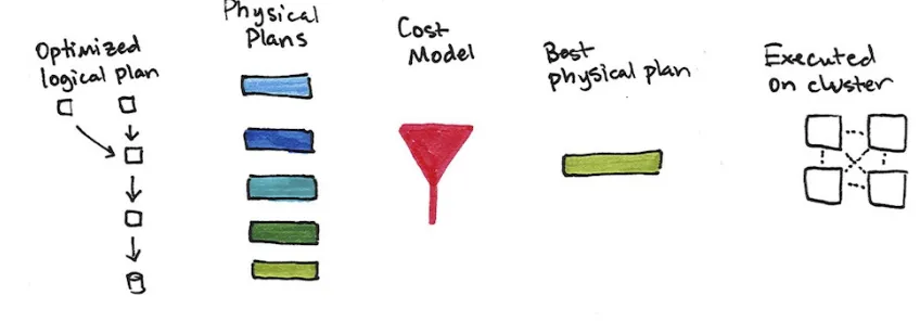
Physical Planning
After successfully creating an optimized logical plan, Spark then begins the physical planning process. The physical plan, often called a Spark plan, specifies how the logical plan will execute on the cluster by generating different physical execution strategies and comparing them through a cost
model. An example of the cost comparison might be choosing how to perform a given join by looking at the physical attributes of a given table (how big the table is or how big its partitions are.)
Execution
Upon selecting a physical plan, Spark runs all of this code over RDDs, the lower-level programming interface of Spark covered in Part III. Spark
Chapter Overview
In the previous chapter we introduced the core abstractions of the Structured API. This chapter will move away from the architectural concepts and towards the tactical tools you will use to manipulate DataFrames and the data within them. This chapter will focus exclusively on single DataFrame operations and avoid aggregations, window functions, and joins which will all be discussed in depth later in this section.
Definitionally, a DataFrame consists of a series of records (like rows in a table), that are of type Row, and a number of columns (like columns in a spreadsheet) that represent an computation expression that can performed on each individual record in the dataset. The schema defines the name as well as the type of data in each column. The partitioning of the DataFrame defines the layout of the DataFrame or Dataset’s physical distribution across the cluster. The partitioning scheme defines how that is broken up, this can be set to be based on values in a certain column or non-deterministically.
Let’s define a DataFrame to work with.
%scala
val df = spark.read.format("json")
.load("/mnt/defg/flight-data/json/2015-summary.json") %python
df = spark.read.format("json")\
.load("/mnt/defg/flight-data/json/2015-summary.json")
We discussed that a DataFame will have columns, and we use a “schema” to view all of those. We can run the following command in Scala or in Python.
df.printSchema()
Schemas
A schema defines the column names and types of a DataFrame. We can either let a data source define the schema (called schema on read) or we can define it explicitly ourselves.
NOTE
Deciding whether or not you need to define a schema prior to reading in your data depends your use case. Often times for ad hoc analysis, schema on read works just fine (although at times it can be a bit slow with plain text file formats like csv or json). However, this can also lead to
precision issues like a long type incorrectly set as an integer when
reading in a file. When using Spark for production ETL, it is often a good idea to define your schemas manually, especially when working with untyped data sources like csv and json because schema inference can vary depending on the type of data that you read in.
Let’s start with a simple file we saw in the previous chapter and let the semi-structured nature of line-delimited JSON define the structure. This data is flight data from the United States Bureau of Transportation statistics.
.schema
Python will return:
StructType(List(StructField(DEST_COUNTRY_NAME,StringType,true), StructField(ORIGIN_COUNTRY_NAME,StringType,true),
StructField(count,LongType,true)))
A schema is a StructType made up of a number of fields, StructFields, that have a name, type, and a boolean flag which specifies whether or not that
column can contain missing or null values. Schemas can also contain other StructType (Spark’s complex types). We will see this in the next chapter when we discuss working with complex types.
Here’s out to create, and enforce a specific schema on a DataFrame. If the types in the data (at runtime), do not match the schema. Spark will throw an error.
%scala
import org.apache.spark.sql.types.{StructField, StructType, StringType val myManualSchema = new StructType(Array(
new StructField("DEST_COUNTRY_NAME", StringType, true), new StructField("ORIGIN_COUNTRY_NAME", StringType, true),
new StructField("count", LongType, false) // just to illustrate flipping this flag ))
val df = spark.read.format("json") .schema(myManualSchema)
.load("/mnt/defg/flight-data/json/2015-summary.json") Here’s how to do the same in Python.
%python
from pyspark.sql.types import StructField, StructType, StringType myManualSchema = StructType([
StructField("DEST_COUNTRY_NAME", StringType(), True), StructField("ORIGIN_COUNTRY_NAME", StringType(), True), StructField("count", LongType(), False)
])
.schema(myManualSchema)\
.load("/mnt/defg/flight-data/json/2015-summary.json")
Columns and Expressions
To users, columns in Spark are similar to columns in a spreadsheet, R
dataframe, pandas DataFrame. We can select, manipulate, and remove columns from DataFrames and these operations are represented as expressions.
To Spark, columns are logical constructions that simply represent a value computed on a per-record basis by means of an expression. This means, in order to have a real value for a column, we need to have a row, and in order to have a row we need to have a DataFrame. This means that we cannot
Columns
There are a lot of different ways to construct and or refer to columns but the two simplest ways are with the col or column functions. To use either of these functions, we pass in a column name.
%scala
import org.apache.spark.sql.functions.{col, column} col("someColumnName")
column("someColumnName") %python
from pyspark.sql.functions import col, column col("someColumnName")
column("someColumnName")
We will stick to using col throughout this book. As mentioned, this column may or may not exist in our of our DataFrames. This is because, as we saw in the previous chapter, columns are not resolved until we compare the column names with those we are maintaining in the catalog. Column and table
resolution happens in the analyzer phase as discussed in the first chapter in this section.
NOTE
Above we mentioned two different ways of referring to columns. Scala has some unique language features that allow for more shorthand ways of referring to columns. These bits of syntactic sugar perform the exact same thing as what we have already, namely creating a column, and provide no performance improvement.
%scala
The $ allows us to designate a string as a special string that should refer to an expression. The tick mark ' is a special thing called a symbol, that is Scala-specific construct of referring to some identifier. They both perform the same thing and are shorthand ways of referring to columns by name. You’ll likely see all the above references when you read different people’s spark code. We leave it to the reader for you to use whatever is most comfortable and maintainable for you.
Explicit Column References
If you need to refer to a specific DataFrame’s column, you can use the col method on the specific DataFrame. This can be useful when you are performing a join and need to refer to a specific column in one DataFrame that may share a name with another column in the joined DataFrame. We will see this in the joins chapter. As an added benefit, Spark does not need to resolve this column itself (during the analyzer phase) because we did that for Spark.
Expressions
Now we mentioned that columns are expressions, so what is an expression? An expression is a set of transformations on one or more values in a record in a DataFrame. Think of it like a function that takes as input one or more column names, resolves them and then potentially applies more expressions to create a single value for each record in the dataset. Importantly, this “single value” can actually be a complex type like a Map type or Array type.
In the simplest case, an expression, created via the expr function, is just a DataFrame column reference.
import org.apache.spark.sql.functions.{expr, col}
In this simple instance, expr("someCol") is equivalent to col("someCol").
Columns as Expressions
Columns provide a subset of expression functionality. If you use col() and wish to perform transformations on that column, you must perform those on that column reference. When using an expression, the expr function can actually parse transformations and column references from a string and can
subsequently be passed into further transformations. Let’s look at some examples.
expr("someCol - 5") is the same transformation as performing
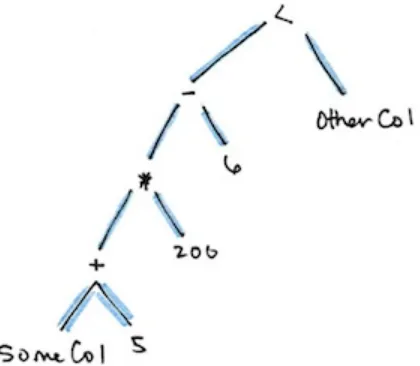
col("someCol") - 5 or even expr("someCol") - 5. That’s because Spark compiles these to a logical tree specifying the order of operations. This might be a bit confusing at first, but remember a couple of key points.
1. Columns are just expressions.
2. Columns and transformations of those column compile to the same logical plan as parsed expressions.
(((col("someCol") + 5) * 200) - 6) < col("otherCol") Figure 1 shows an illustration of that logical tree.
This might look familiar because it’s a directed acyclic graph. This graph is represented equivalently with the following code.
%scala
import org.apache.spark.sql.functions.expr expr("(((someCol + 5) * 200) - 6) < otherCol") %python
from pyspark.sql.functions import expr
expr("(((someCol + 5) * 200) - 6) < otherCol")
This is an extremely important point to reinforce. Notice how the previous expression is actually valid SQL code as well, just like you might put in a SELECT statement? That’s because this SQL expression and the previous DataFrame code compile to the same underlying logical tree prior to
Overview of the Structured APIs chapter.
Accessing a DataFrame’s Columns
Sometimes you’ll need to see a DataFrame’s columns, you can do this by doing something like printSchema however if you want to programmatically access columns, you can use the columns method to see all columns listed.
spark.read.format("json")
Records and Rows
In Spark, a record or row makes up a “row” in a DataFrame. A logical record or row is an object of type Row. Row objects are the objects that column
expressions operate on to produce some usable value. Row objects represent physical byte arrays. The byte array interface is never shown to users because we only use column expressions to manipulate them.
You’ll notice collections that return values will always return one or more Row types.
Note
we will use lowercase “row” and “record” interchangeably in this chapter, with a focus on the latter. A capitalized “Row” will refer to the Row object. We can see a row by calling first on our DataFrame.
Creating Rows
You can create rows by manually instantiating a Row object with the values that below in each column. It’s important to note that only DataFrames have
schema. Rows themselves do not have schemas. This means if you create a Row manually, you must specify the values in the same order as the schema of the DataFrame they may be appended to. We will see this when we discuss creating DataFrames.
%scala
import org.apache.spark.sql.Row
val myRow = Row("Hello", null, 1, false) %python
from pyspark.sql import Row
myRow = Row("Hello", None, 1, False)
Accessing data in rows is equally as easy. We just specify the position.
However because Spark maintains its own type information, we will have to manually coerce this to the correct type in our respective language.
For example in Scala, we have to either use the helper methods or explicitly coerce the values.
%scala
myRow(0) // type Any
myRow(0).asInstanceOf[String] // String myRow.getString(0) // String
myRow.getInt(2) // String
There exist one of these helper functions for each corresponding Spark and Scala type. In Python, we do not have to worry about this, Spark will
automatically return the correct type by location in the Row Object.
myRow[0] myRow[2]
DataFrame Transformations
Now that we briefly defined the core parts of a DataFrame, we will move onto manipulating DataFrames. When working with individual DataFrames there are some fundamental objectives. These break down into several core operations.
We can add rows or columns We can remove rows or columns
We can transform a row into a column (or vice versa)
Creating DataFrames
As we saw previously, we can create DataFrames from raw data sources. This is covered extensively in the Data Sources chapter however we will use them now to create an example DataFrame. For illustration purposes later in this chapter, we will also register this as a temporary view so that we can query it with SQL.
%scala
val df = spark.read.format("json")
.load("/mnt/defg/flight-data/json/2015-summary.json")
We can also create DataFrames on the fly by taking a set of rows and converting them to a DataFrame.
%scala
import org.apache.spark.sql.Row
import org.apache.spark.sql.types.{StructField, StructType, StringType, LongType} val myManualSchema = new StructType(Array(
new StructField("some", StringType, true), new StructField("col", StringType, true),
new StructField("names", LongType, false) // just to illustrate flipping this flag ))
val myRows = Seq(Row("Hello", null, 1L))
val myRDD = spark.sparkContext.parallelize(myRows)
Note
In Scala we can also take advantage of Spark’s implicits in the console (and if you import them in your jar code), by running toDF on a Seq type. This does not play well with null types, so it’s not necessarily recommended for
production use cases.
%scala
val myDF = Seq(("Hello", 2, 1L)).toDF() %python
from pyspark.sql import Row
from pyspark.sql.types import StructField, StructType,\ StringType, LongType
myManualSchema = StructType([
StructField("some", StringType(), True), StructField("col", StringType(), True), StructField("names", LongType(), False) ])
myRow = Row("Hello", None, 1)
myDf = spark.createDataFrame([myRow], myManualSchema) myDf.show()
Now that we know how to create DataFrames, let’s go over their most useful methods that you’re going to be using are: the select method when you’re working with columns or expressions and the selectExpr method when
you’re working with expressions in strings. Naturally some transformations are not specified as a methods on columns, therefore there exists a group of
Select & SelectExpr
Select and SelectExpr allow us to do the DataFrame equivalent of SQL queries on a table of data.
SELECT * FROM dataFrameTable
SELECT columnName FROM dataFrameTable
SELECT columnName * 10, otherColumn, someOtherCol as c FROM dataFrameTable In the simplest possible terms, it allows us to manipulate columns in our
DataFrames. Let’s walk through some examples on DataFrames to talk about some of the different ways of approaching this problem. The easiest way is just to use the select method and pass in the column names as string that you
would like to work with.
%scala
You can select multiple columns using the same style of query, just add more column name strings to our select method call.
"DEST_COUNTRY_NAME",
As covered in Columns and Expressions, we can refer to columns in a number of different ways; as a user all you need to keep in mind is that we can use them interchangeably.
%scala
import org.apache.spark.sql.functions.{expr, col, column} df.select(
from pyspark.sql.functions import expr, col, column df.select(
expr("DEST_COUNTRY_NAME"), col("DEST_COUNTRY_NAME"), column("DEST_COUNTRY_NAME"))\ .show(2)
One common error is attempting to mix Column objects and strings. For example, the below code will result in a compiler error.
df.select(col("DEST_COUNTRY_NAME"), "DEST_COUNTRY_NAME")
can refer to a plain column or a string manipulation of a column. To illustrate, let’s change our column name, then change it back as an example using the AS keyword and then the alias method on the column.
%scala
DEST_COUNTRY_NAME as destination FROM
dfTable
We can further manipulate the result of our expression as another expression.
%scala df.select(
expr("DEST_COUNTRY_NAME as destination").alias("DEST_COUNTRY_NAME" )
%python df.select(
expr("DEST_COUNTRY_NAME as destination").alias("DEST_COUNTRY_NAME" )
Because select followed by a series of expr is such a common pattern, Spark has a shorthand for doing so efficiently: selectExpr. This is probably the most convenient interface for everyday use.
%scala
df.selectExpr(
"DEST_COUNTRY_NAME as newColumnName", "DEST_COUNTRY_NAME")
df.selectExpr(
"DEST_COUNTRY_NAME as newColumnName", "DEST_COUNTRY_NAME"
).show(2)
This opens up the true power of Spark. We can treat selectExpr as a simple way to build up complex expressions that create new DataFrames. In fact, we can add any valid non-aggregating SQL statement and as long as the columns resolve - it will be valid! Here’s a simple example that adds a new column withinCountry to our DataFrame that specifies whether or not the destination and origin are the same.
%scala
df.selectExpr(
"*", // all original columns
"(DEST_COUNTRY_NAME = ORIGIN_COUNTRY_NAME) as withinCountry" ).show(2)
%python
df.selectExpr(
"*", # all original columns
"(DEST_COUNTRY_NAME = ORIGIN_COUNTRY_NAME) as withinCountry") .show(2)
%sql SELECT *,
(DEST_COUNTRY_NAME = ORIGIN_COUNTRY_NAME) as withinCountry FROM
dfTable
Now we’ve learning about select and select expression. With these we can specify aggregations over the entire DataFrame by leveraging the functions that we have. These look just like what we have been showing so far.
%scala
df.selectExpr("avg(count)", "count(distinct(DEST_COUNTRY_NAME))" %sql
SELECT
avg(count),
count(distinct(DEST_COUNTRY_NAME)) FROM
Converting to Spark Types (Literals)
Sometimes we need to pass explicit values into Spark that aren’t a new column but are just a value. This might be a constant value or something we’ll need to compare to later on. The way we do this is through literals. This is basically a translation from a given programming language’s literal value to one that Spark understands. Literals are expressions and can be used in the same way.
%scala
from pyspark.sql.functions import lit df.select(
expr("*"),
lit(1).alias("One") ).show(2)
In SQL, literals are just the specific value.
%sql