39
2
Demand
C O N C E P T S
● Determinants of Demand ● Demand Schedule
● Demand Curve ● Demand Function
● Normal/Superior Good ● Inferior Good
● Substitute Goods ● Complementary Goods
● Veblen Effect ● Veblen Good
● Bandwagon Effect ● Snob Effect
● Network Externality ● Market Demand
● Change in Quantity Demanded versus Change in Demand ● Price Elasticity of Demand
● Arc Elasticity of Demand ● Point Elasticity of Demand
● Elastic Demand ● Inelastic Demand
● Unitarily Elastic ● Perfectly Inelastic
● Perfectly Elastic ● Income Elasticity
● Cross Price Elasticity ● Product Line
M
r Goyal was thinking of selling two 100-square-yard plots that he owned in his hometown at Rs 10 lakh each, in order to pay for his son’s education in America (costing Rs 20 lakh). Suddenly, some IT indus-tries moved into the town as the state government began to develop it as an ‘IT Park’. Demand for real estate skyrocketed. Within six months one plot fetched Rs 20 lakh. Mr Goyal had to sell only one plot to finance his son’s education abroad.In 1973, the OPEC (Organization of Petroleum Exporting Countries) collec-tively curtailed the production of oil drastically. The supply of oil in the world market fell so much that the price of oil quadrupled within one year.1The world economic scenario has since then changed permanently.
The preceding examples illustrate how market-forces work. In the first exam-ple, there was an increase in demand, which resulted in a land-price hike. In the second example, the price of oil soared because of a reduction in supply. ‘Demand’ and ‘Supply’ are very important concepts in economics, which help us to under-stand and explain simple as well as complicated situations. In this chapter and in Chapters 4, 5 and 6, we will learn about demand.
INDIVIDUAL DEMAND FOR A COMMODITY/SERVICE
Suppose each month, your parents give you Rs 1,500 as your stipend, which you spend on food, snacks, stationery, movies, clothes and so on. In this context, think of your demand for ice-cream in a month and ask yourself what factors determine how many ice-cream cones you would buy within a month. You may come up with the following factors:
PRICE OF ICE-CREAM CONES
Assume that all ice-cream cones are of the same kind and quality. Suppose they become more expensive than before—from Rs 15 to Rs 30 a piece. Unless you can-not live without eating so many ice-creams per month, the effect would be that you would consume less ice-cream than before. (Perhaps you will switch partly to a substitute product, saykulfi.)
YOUR MONTHLY STIPEND
Suppose, as a reward for having done very well in the exams, your parents raise your stipend from Rs 4,000 to Rs 5,000. You would probably spend more on clothing, entertainment and food (including ice-cream), that is, the effect would be that you would demand more ice-cream.
PRICE OF KULFI
Suppose that for some very unusual reason, kulfi becomes very cheap—Rs 4 per plate instead of Rs 10. (Your stipend remains unchanged at Rs 4,000.) Would you buy as many ice-creams as before? Given that you do like kulfi(although perhaps not as much as ice-cream), you would probably eat more kulfiand less ice-cream.
WEIGHT CONSCIOUSNESS
Suppose you have become very weight conscious lately. Since ice-cream is ‘fattening,’ you may consume less ice-cream than before even when there is no change in prices or your stipend.
FUTURE PRICE EXPECTATION
Imagine a rumour saying that within a matter of one week, ice-cream will be dou-bly expensive because of supply problems. If such a rumour spreads, many of you would dash to buy ice-cream now and store them in the refrigerator. In other words, your presentdemand for ice-cream is affected by futureprice expectation, while there is no change in the stipend or in any price.
We have listed above most, if not all, of the factors that may affect your demand for ice-cream.2 We can generalise from this. Interpret the price of ice-cream as ‘own price’ the price of kulfias the ‘price of a related good,’ monthly stipend as ‘income’ and weight-consciousness as ‘taste’ in the sense that it has changed your ‘effective’ taste for ice-cream.
Now think of consumables like clothing, household items and other types of food. We can say that the demand for a product by an individual or a household depends on:
(a) own price, (b) income,
(c) prices of related goods, (d) taste and
(e) future price expectations.
The term ‘income’ refers to the total expenditure on all the different goods you may wish to purchase in a given time period. Note that such a characterisation applies not just to goods (commodities) but also services.3
The question now is how, in general, these factors affect the quantity demanded of a product or a service.
2There may be other factors. For instance, a change in weather may affect your demand for ice-cream.
Own Price
The effect of own price is captured through what is called the law of demandin economics. It states that, other things remaining unchanged, the quantity demanded of a product by a consumer falls as its own price increases. This is quite intuitive—saying that if a product becomes more (or less) expensive, you would buy less (or more) of it. Note that: (i) ‘other things’ refers to other factors affecting demand like income and prices of related goods, and (ii) the law applies in the context of a given area and within a given time period.
Table 2.1 presents a numerical example of this law and is interpreted as follows. If the price of an ice-cream cone were Rs 10, Sunita would buy 50 cones; if it were Rs 12, she would buy 40 cones and so on—although at any given point of time (and space) there is a uniform price of ice-cream. The law of demand presented in a table is called a Demand Schedule. Table 2.1 is a demand schedule.
The numbers in Table 2.1 are graphed in Figure 2.1(a), in which (own) price is measured on the y-axis and quantity demanded along the x-axis. This is the
Table 2.1 Demand for Ice-cream by Sunita during Summer Months
Own Price in Rs Quantity Demanded of Ice-cream
demand curve corresponding to the demand schedule in Table 2.1. In general, demand curveis a graphical representation of the law of demand, measuring the inverse relationship between own price and the quantity demanded.4A demand
curve is typically illustrated as a smooth downward sloping curve, as shown in Figure 2.1(b). For example, at the price p0, the quantity demanded is q0and the consumer is at the point Aon the demand curve. At a higher price p1, the quantity demanded is less (equal to q1) and the consumer is at point B. And so on.
The law of demand holds generally but not universally. There are exceptions and we will learn about these as we go along. But unless mentioned explicitly, it is presumed that the law holds and the demand curve is downward sloping.
Income
Suppose the income of a consumer rises and other things (including the own price) remain the same. Would she buy more or less of a particular good?
Normally one would buy more. But it may not be true for all goods. As an example, suppose your income (or stipend) is low. You are probably consuming a fair amount of low-priced snacks like peanuts and biscuits, which you do not like as much as, say, ice-cream, but you buy them because that is mostly what you can afford with your low income. However, if your income rises, it is likely that you will buy less of peanuts and biscuits and more of ice-cream because you are in a position to afford what you like more.
In this example, as income increases, the demand for ice-cream increases and that for peanuts falls. In general, if the demand for a product increases with income, it is called a superior or a normal good. But, if less of a good is demanded as income increases, it is called an inferior good. See Clip 2.1 for a discussion of inferior goods.
Clip 2.1: Which Goods are Inferior in Reality?
Typically, certain cereals are inferior goods. For instance, in most parts of the world, maize, also called corn, has been found to be an inferior good. Rosegrant, Agcaoili-Sombilla and Perez (1995) report that, in Philippines, a 1 per cent increase in income leads to a 0.15 per cent decrease in white maize consumed. Minot and Goletti (2000) find that in Vietnam, even rice is an infer-ior good given that an increase in income is associated with a decrease in the amount of rice consumed. According to Mckenzie (2002), tortillas in Mexico are inferior goods.
Are cereals inferior goods in India? Most studies, like Radhakrishna and Ravi (1994), Bhalla, Hazell and Kerr (1999) and others, find that they are not. However, according to Kumar (1998), they are; this result is an exception.
4An inverse relationship between two entities means that, as one entity increases, the other decreases.
The effect of income on quantity demanded is illustrated in Figure 2.2. Panels (a) and (b) respectively show a normal good and an inferior good. In both panels, D0D0 represents the original demand curve andD1D1 the new demand curve after an increase in income. Panel (a) shows that at price p0, for instance, the quantity demanded originally was A0. At a higher income but at the same price p0, the quantity demanded is B0, which is greater than A0. Similarly, at price p1, the original quantity demanded was A1, whereas the new quantity demanded with higher income is B1. The same pattern holds at any particular price—quantity demanded is greater with higher income—which exactly defines a normal or a superior good. We can then say that, for a normal or superior good, an increase in income shifts the demand curve to the right; by the same logic, a decrease in income shifts the demand curve to the left.
Panel (b) of Figure 2.2 shows the opposite for an inferior good—an increase (or a decrease) in income shifts the demand curve of such a good to the left (or right).
Figure 2.2 Effect of an Increase in Income on Demand References
Bhalla, G. S., P. Hazell and J. Kerr. 1999. ‘Prospects for India’s Cereal Supply and Demand to 2020’. Food, Agriculture and Environment Discussion Paper 29, Washington, DC: International Food Policy Research Institute.
Kumar, P. 1998. ‘Food Demand and Supply Projections for India’. Agricultural Economics Policy Paper 98-01, New Delhi: Indian Agricultural Research Institute.
Mckenzie, D. 2002. ‘Are Tortillas a Giffen Good in Mexico?’, Economics Bulletin, 15(1): 1–7. Minot, N. and F. Goletti. 2000. ‘Rice Market Liberalization and Poverty in Vietnam’. Research
Report No. 114, Washington, DC: International Food Policy Research Institute.
NUMERICAL EXAMPLE 2.1
Table 2.2 is the original market demand schedule of Mr Yamada for a particular kind of fish. Suppose that Mr Yamada’s income has increased and for him the fish in question is a normal good. Fill in the blanks in the 3rdcolumn, which will
rep-resent a shift of Mr Yamada’s demand curve for this fish.
Since this fish is a normal good for Mr Yamada, an increase in income will induce him to demand more at each price. An example of this is given in Table 2.3. Notice that, along column 3, the quantity demanded at each price is higher as compared to column 2. (Yet along column 3 the quantity demanded falls as the price increases.) If we plot the old and the new demand schedules, the latter will be positioned to the right of the former—as in Figure 2.2(a).
PRICES OF RELATED GOODS
In taste, two goods can be related to each other in two ways: they may be substitutes for each other or one may be a complement to the other. In drinks, tea and coffee are substitutes for each other. In meat, chicken and mutton are substitutes. In staple food, rice and chapattiare substitutes. But consider tea and sugar. Sugar is a com-plement to tea—if you consume more tea, you consume more sugar (unless, of course, you are diabetic).5Substitutability or complementarity is not restricted to
Table 2.2 Original Market Demand Schedule of Mr Yamada (Numerical Example 2.1)
Price in Yen Mr Yamada’s His Demand for Fish after (the Japanese currency) Demand for Fish an Increase in Income
100 10 ?
200 7 ?
300 6 ?
400 5 ?
500 3 ?
600 1 ?
Table 2.3 Mr Yamada’s Demand after an Increase in Income (Numerical Example 2.1)
Price in Yen Mr Yamada’s His Demand for Fish after (the Japanese currency) Demand for Fish an Increase in Income
100 10 13 (>10)
200 7 10 (>7)
300 6 9 (>6)
400 5 6 (>5)
500 3 4 (>2)
600 1 2 (>1)
food or drinks only. For instance, the demand for auto mechanic services is com-plementary to the demand for automobiles.
If two goods are related in taste it is natural that a change in the price of one good will affect the demand for the other. This is called the cross price effect, defined as the effect of a change in the price of one good on the demand for another.
Consider the demand for tea. How will it be affected by an increase in the price of coffee? It would increase, since a substitute good is now costlier. This implies that, as the price of coffee increases, the demand curve for tea shifts to the right (that is, at any given price of tea, more tea will be demanded at a higher coffee price). Thus, an increase (or a decrease) in the price of a substitute good shifts the demand curve of a product to the right (or left). This is exhibited in Figure 2.3(a). Now ask yourself how an increase in the price of tea would affect the demand for sugar. Tea consumption will fall and so will the demand for sugar. It is oppo-site of what happens when the price of a substitute good increases. Thus, an increase (or a decrease) in the price of a complementary good shifts the demand curve of a product to the left (or right). This is shown in Figure 2.3(b).
Taste
A person’s taste for a product changes for various reasons. When younger, you very much disliked bitter guord; but now your natural dislike may not be that intense. A change in taste may occur even when there is no change in your natural liking. For instance, because of health problems, you may be consuming less chocolate and ice-cream, even though your natural liking for them remain as strong as ever. Taste changes can happen with respect to non-food products too.
How does a taste change affect the demand for a commodity? It is quite simple: a favourable (or an unfavourable) change in taste for a product increases (or decreases) the demand and hence shifts the demand curve to the right (or left).
Price
D0
D0 D1
D1
Quantity Demanded
0
(a) Price Increase of a Substitute Good
(b) Price Increase of a Complementary Good Price
D0 D1
D1
Quantity Demanded
0
D0
Expectations
Suppose there is an unexpected weather forecast that a huge cyclone is going to hit your town in the next three days. People then anticipate that there will be sup-ply problems for many daily usable items during and immediately after the cyclone and hence these items will be much more costly. This induces them to rush to the market now and buy things like oil, bread and potatoes in bulk. Thus it is a situation where there is no change in income, own price, prices of related goods or tastes, yet there is an increase in the currentdemand for some products.
We can then say that an increase (or a decrease) in the expected price of a product increases (or decreases) the current demand for it and shifts its current demand curve to the right (or left).
Other Factors
There are still other factors that can influence a person’s demand for a commod-ity. For example, some people, in order to impress others (and possibly them-selves), tend to buy more of a good when it becomes more expensive. You can think of this as a (strange) change in taste because of a change in price. This is called a Veblen effectand the good in question is called a Veblen good.6Veblen goods are ‘conspicuous goods’, which others may look upon with some envy— like a branded car or a fancy jacket. As the quantity demanded increases with price, the law of demand does not obviously hold for a Veblen good and for a per-son whose behaviour is subject to the Veblen effect.
There may be a bandwagon effect,that is, if others start to use a product in a big way, it becomes fashionable and so you go for it too without looking at its merit. In other words, you ‘follow the crowd’.
There can also be a snob effect, referring to a situation where you want to be different from others for the sake of being different, that is, you ‘go against the crowd’. If more people buy something, your demand for it falls. This is the oppo-site of the bandwagon effect.
Still another effect can be in the form of a network externality, defined as a change in the benefit to a person when the number of other individuals using it increases. For instance, if your friends, relatives and colleagues do not use e-mail, your demand for e-mail will be small. But if they all start to use e-mail, your demand for e-mail will increase. Thus a person’s benefit increases with the size of the network and, therefore, an increase in the number of consumers in a network increases the individual demand for the product or service. Note that it is some-what similar to but not the same as the bandwagon effect, which makes you ‘go’ for the product without looking at its merit.
The opposite can also happen—a person’s benefit may decrease with the number of users in a network. Consider using the bus service in a city. If the number of bus-riders increases and the buses are overcrowded, it may lower your benefit from a
bus-ride and induce you to use less of it. This is a case of negative externality, whereas the e-mail example was a case of positive externality. Unless specified, the convention is that network externality refers to the case of a positive externality.
Mathematically Speaking
The Demand Function
The dependence of demand for a particular good on several factors can be expressed algebraically in the form of a demand function. Consider the demand for, say, good A. Use the following notations: qA≡the quantity demanded of good
A, pA≡the own price, p
B, pC≡prices of related goods (there can be other related
goods), M ≡the income and T ≡other factors. The demand function for good A
can be written as a mathematical relation:
qA=f(p
A, pB, pC, M, T).
How different factors affecting the quantity demanded of a good determine the properties of the demand function f.
The law of demand implies that, other things remaining constant, as pAchanges, qAchanges in the opposite direction. Hence, the partial derivative
∂f/∂p
A, which is same as ∂qA/∂pA, is negative in sign. Suppose good Bis a
sub-stitute for good A. Then, a change in pBcauses qAto change in the same direc-tion. Therefore, ∂f/∂p
B > 0. Similarly, if good A is complementary to good C,
∂f/∂p
C<0.
The partial derivative with respect to Mdepends on whether good Ais normal or inferior. By applying similar reasoning, ∂f/∂Mis positive or negative if good
Ais normal or inferior respectively. The sign of ∂f/∂Tdepends on the nature of T.
Suppressing the ‘other factors’ T, an example of a demand function will be:
qA=100 −2p
A+0.5pB−pC+1.5M.
It means, for example, that if there is a unit increase in own price, the quantity demanded will fall by 2 units. For instance, let pA be measured in hundreds of rupees. Then, starting from an initial value, if pAincreases by Rs 100, then qAwill decrease by 2 units.
If we are only concerned with changes in own price, that is, pB, pCand M are unchanged, for notational simplicity, we can also suppress them and write the demand function very simply as:
qA=f(p
A).
As an example, we can write:
qA=200 −2p
A.
MARKET DEMAND
So far we have analysed the demand for a particular good by a single individual, family or household. Market demandis the total demand by all individuals
com-prising the entire market.7
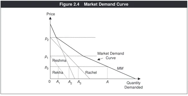
As a simple example, let there be only three individuals in the market: Rekha, Reshma and Rachel. Figure 2.4 depicts their individual demand curves for ice-cream, marked by the respective dotted lines. (Reshma’s demand curve is partly hidden; it extends all the way up to the y-axis.) It is presumed for simplicity that the demand for ice-cream can be measured continuously as points on a line. For instance, at price p0, Rekha demands 0A1, Reshma 0A2and Rachel 0A3. Then the quantity demanded in the market at price p0equals 0A1+0A2+0A3. This sum is
equal to 0A, where the point Ais marked on the curve MM. Other points on this curve are obtained by similar exercises at other prices.8The MMcurve is then the
market demand curve.9
7By ‘market,’ one could mean the entire city, province, region, country or even the whole world. It depends on the context
of the analysis.
8Note that at any price equal to or greater than p
2, the quantity demanded of ice-cream by Rekha and Rachel is zero. Thus
the total quantity demanded is same as the quantity demanded by Reshma only. Similarly, at any price between p1and p2,
the quantity demanded by Rekha is zero. Hence the total quantity demanded equals the sum of quantities demanded by Reshma and Rachel. At any price below p1, all three individuals demand positive quantities and these are added to obtain
the total quantity demanded in the market.
9Note that if there were 10 or 10 lakh individuals in the market, we would have done the same thing in principle, that is,
added up the quantities demanded by all individuals in the market at each price.
Price
Quantity Demanded Market Demand
Curve
Rekha Reshma
Rachel 0
p1
MM
A2 p2
p0
A3 A
A1
In obtaining the market demand curve, essentially, the quantities measured along the horizontal, x-axis are added up. Thus we can say that the market demand curve is the horizontal or lateral summation of individual demand curves.
Mathematically, if there are, say, Hfamilies, denoted by 1, 2, 3, …, H, and their
demand functions are f1(p), f2(p) and so on, the market demand function is given by f1(p) +f
2(p) + … +fH(p).
What are the factors that can shift a market demand curve? Since it is based on individual demand curves and the number of individuals constituting the market, these factors are:
(a) income levels of individuals, that is, income distribution across consumers in the market,
(b) prices of related goods,
(c) tastes of individuals (that is, distribution of tastes) and (d) the number of individuals or consuming units in the market.
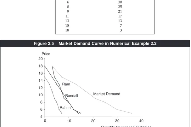
NUMERICAL EXAMPLE 2.2
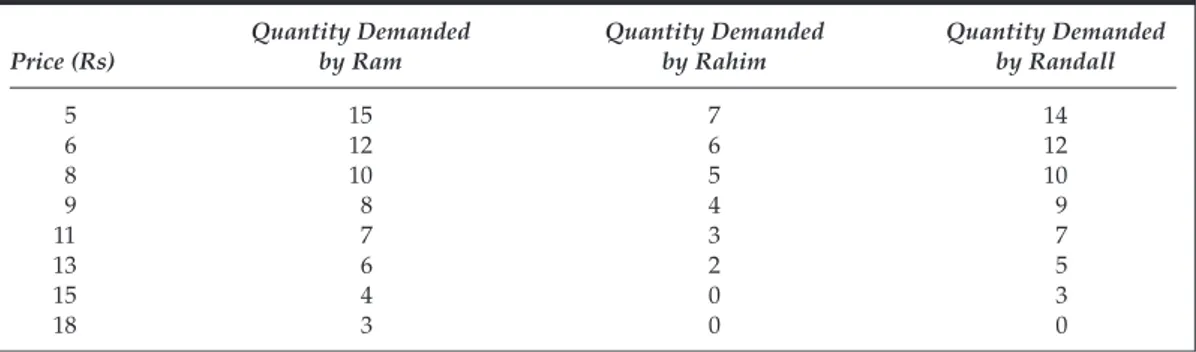
Suppose there are three individuals in the market: Ram, Rahim and Randall. Their individual demand schedules for apples are given in Table 2.4. For example, at the price of Rs 9, Rahim consumes (demands) 4 apples. Derive the market demand schedule and plot individual and market demand curves.
At each price, we sum up the individual quantities demanded. Thus at price equal to Rs 5, the total or market quantity demanded =15 +7 +14 =36. At price
Rs 6, it is equal to 12 + 6 +12 =30, and so on. Table 2.5 is the market demand
schedule.
Figure 2.5 depicts the individual curves and the market demand curve in this numerical example.
Table 2.4 Individual Demand Schedules (Numerical Example 2.2)
Quantity Demanded Quantity Demanded Quantity Demanded
Price (Rs) by Ram by Rahim by Randall
5 15 7 14
6 12 6 12
8 10 5 10
9 8 4 9
11 7 3 7
13 6 2 5
15 4 0 3
CHANGE IN QUANTITY DEMANDED VERSUS
CHANGE IN DEMAND
Think for a moment about how we have organised the effects of various factors on demand for a particular commodity (by an individual or the entire market). First, the effect of a change in the own price is characterised by the law of demand and depicted as the demand curve. Second, the effects of changes in other factors like income, prices of related goods and taste are seen through a shift in the demand curve.
Having understood this, we can differentiate the two terms in the title of this sec-tion. Refer back to Figure 2.1(b): suppose the own price changes from p0to p1, then the consumer ‘moves’, so-to-speak, from point Ato point Bon the same demand curve. This is called a change in quantity demanded—meaning a movement along a given demand curve due to a change in the own price. On the other hand,
Table 2.5 Market Demand Schedule (Numerical Example 2.2)
Price (Rs) Total Quantity Demanded of Apples
5 36
6 30
8 25
9 21
11 17
13 13
15 7
18 3
4 6 8 10 12 14 16 18 20
0 10 20 30 40
Market Demand Ram
Rahim Randall Price
Quantity Demanded of Apples
achange in demandrefers to a change in the whole demand schedule or curve, which is same as a shift of the demand curve that occurs due to a change in other factors such as income, prices of related goods or taste. In other words, the first term refers to the movement alonga demand curve and the second to a movement ofit.
ELASTICITY
So far, we have learnt how different factors qualitativelyaffect the demand for a particular good—the directionof change in the quantity demanded of a good—as the own price, the prices of related goods, income or tastes change. We now learn about concepts of ‘elasticity’ that aim to quantifythe responsiveness of the quan-tity demanded of a good to changes in the various factors.
Price Elasticity of Demand
It measures the response of the quantity demanded to a change in the own price and is defined by:
(2.1)
We know from the law of demand that the own price and the quantity demanded change in opposite ways. Thus the percentage change in the quantity demanded bears a sign, which is the opposite of that in own price, implying that the ratio of the two percentage changes is negative. Hence the negative sign in front of the formula given in (2.1) makes ep positive. Strictly speaking, ep gives the absolutevalue of the price elasticity, which is commonly (and loosely) called ‘price elasticity.’10By definition, the greater the responsiveness of the quantity demanded for the same proportionate change in price, the higher is the price elasticity.
MEASUREMENT
There are alternative methods to measure ep. The percentage method is one of these.
This method directly applies the formula (2.1). Let, originally, the price of a product be p0, at which the quantity demanded is equal to q0. Let the price change to p1 and, accordingly (along the demand curve), let the quantity demanded change to q1. Then the percentage changes in the own price and in the quantity demanded have the following expressions respectively:
p p p
q q q
1 0
0
1 0
0
100 100
−
× ; − × .
ep = −
% change in quantity demanded % change in the own price ..
The first one goes in the denominator (2.1) and the second in its numerator. Hence,
(2.2)
In economics, a change in something is typically denoted by the greek letter Δ
(pronounced Delta). For example, Δqdwould denote the change in the quantity demanded, equal to q1−q0, and, similarly Δpwould denote p1−p0. Using this
nota-tion, we can also write (2.1) as
(2.3)
A numerical example that uses (2.2) or (2.3) is given below.
NUMERICAL EXAMPLE 2.3
Renu used to consume 10 ice-creams a month when the price of an ice-cream was Rs 12. Ice-cream has become more expensive with Rs 15 a piece. Renu now con-sumes 8 ice-creams a month. What is the epof demand for ice-cream by Renu?
The original price and quantity are: p0=12 and q0=10. The new price and
quan-tity are: p1=15 and q1=8. Thus the percentage change in price =100 × (15 −12)/12.
Similarly, the percentage change in the quantity demanded = 100 × (8 −10)/10.
Applying (2.2) or (2.3),
(2.4)
Arc Elasticity
There is, however, a problem with the percentage method. Consider the above numerical example by regarding the new price and quantity as the old price and quantity respectively, and the old price and quantity as the new price and quantity respectively. Thus, let p0=15, q0=8, p1=12 and q1=10. Since the concept of
elas-ticity refers to the magnitude of the response of the quantity demanded to a price change, the order between which is the old and which is the new price-quantity combination should not ideally matter. But, unfortunately, it does. Apply (2.2) or (2.3) to this example and you will find that ep is not what is given in (2.4). It is equal to 1.25.11
It is not hard to see why this difference is arising. It is because the denominator of the percentage change of price or quantity is sensitive to the original price or quantity. To get around this problem, a compromise is done. Instead of p0in the
denominator of the percentage change of price, we take (p0+p1)/2, that is, the aver-age of the original price and the new price. Similarly q0in the denominator of the percentage change in quantity is replaced by (q0+q1)/2. Then the formula becomes:
(2.5)
This is called the arc elasticity. According to this measure, the computed price elasticity is independent of the original price-quantity combination. In the Numerical Example 2.3, the arc elasticity is equal to 1.00.
NUMERICAL EXAMPLE 2.4
Arup was buying 20 music CDs when the price of a CD was Rs 200. Now the price has come down to Rs 150 and he is buying 30 CDs. (The quality of CDs and the number of songs in each CD are the same.) What is the arc elasticity of demand for music CDs by Arup?
Here the original price and quantity demanded are: p0=200 and q0=20. The new price and quantity demanded are: p1= 150 and q1=30. Thus p0+ p1= 350, q0+q1=50, p1−p0= −50, and q1−q0=10. Applying the formula given in (2.5), the arc elasticity is equal to 1.4.
Geometric Method and Point Elasticity
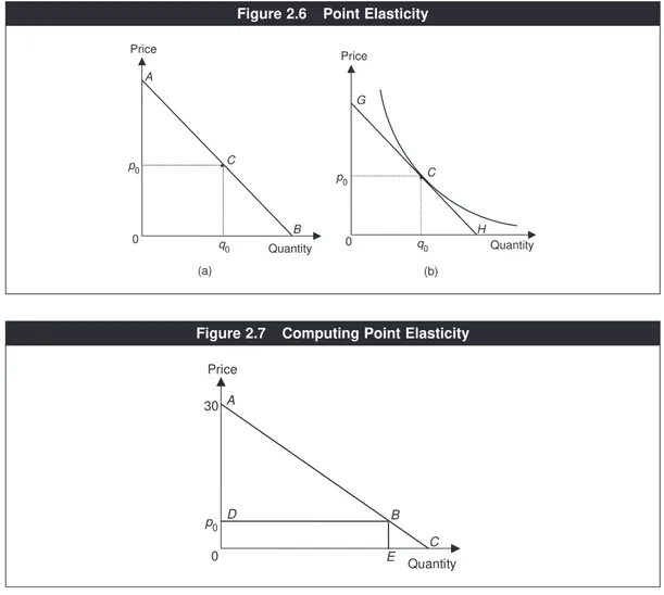
Arc elasticity is an approximate formula, appropriate when the price change is not small. When the price change is very small, we can use a graphical formula or a geometric method. This is illustrated in Figure 2.6.
Consider Panel (a). The demand curve is a straight line intersecting the axes at Aand B. Suppose, initially the price is p0. A consumer is demanding the amount q0, that is, she is at point C on the demand line. Then, as shown mathematically in Appendix 2A, epis equal to BC/CA(the ratio of the lower segment to the upper segment of the line AB).12
If the demand curve is not a straight line, it is a bit more complicated but essen-tially the same. Suppose the demand curve looks like the downward sloping curve shown in panel (b) and we are to compute the price elasticity at the price p0. Now, draw the tangent of the demand curve at the price where the elasticity is to be computed. At p0, it is GH. For a very small price change around p0, epturns out to be equal to HC/CG(again the ratio of the lower to the upper segment). This is also proven in Appendix 2A.
− − +
+ −
( )( )
( )( ).
q q p p
q q p p
1 0 0 1
0 1 1 0
12Note that if we consider a price, which is higher, this ratio will be higher, which means that the higher the price, the
This geometry-based formula is called point elasticity, wherein the word ‘point’ refers to a small variation. In general, the point elasticity at a given price is equal to the ratio of the lower segment to the upper segment of the demand line at that price or the same ratio on the tangent of the demand curve at that price.
NUMERICAL EXAMPLE 2.5
Suppose the demand curve for a product is a straight line as shown in Figure 2.7. Its intercept on the price axis equals 30. Calculate the point elasticity at the pricep0, where p0=9.
Since p0 = 9, we have BE = 0D = 9 and AD = 0A− 0D= 30 − 9 = 21. Hence
BE/AD = 9/21 = 3/7. The triangles BEC and ADB are similar. Thus BE/AD =
BC/AB. Since BE/AD = 3/7, we have the measure of point elasticity (BC/AB)
equal to 3/7.
A
B
Quantity
p0 C
q 0
(a) (b)
Price
Quantity
Price
q0 p
0
C G
H 0
0
• •
Figure 2.6 Point Elasticity
A
D p0
C Price
Quantity
0 E
B 30
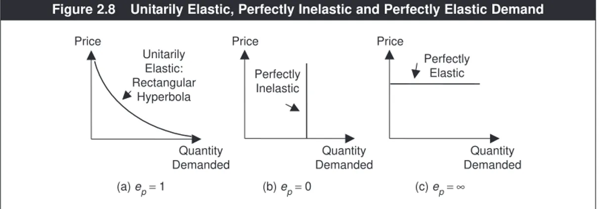
Elastic and Inelastic Demand
These concepts relate to the magnitude of the price elasticity. If ep>1, we say that
the product demand is elastic. Typical examples are luxury items like branded shoes, jewelry and food in a posh hotel. Luxury goods are relatively ‘dispensable’, not essential. Therefore, the quantity demanded of such products can vary a lot, implying that the price elasticity of these goods typically exceeds one. On the other hand, if ep< 1, we say that the demand is inelastic. Necessary goods like
basic food and clothing items fall into this category. Since these are essential, the demand for them is relatively insensitive to price changes. In the intermediate case of ep = 1, the demand for the product is said to be unitarily elastic; the
demand is neither elastic nor inelastic. If ep=1, the demand curve has a particular
mathematical shape called rectangular parabola, as shown in Figure 2.8(a), which is asymptotic to both axes.
There are two other special cases. If ep=0, then the product demand is said to
be perfectly inelastic. This holds when there is no change in quantity demanded
as price changes, that is, the product is absolutely essential to the consumer. A very bad case of addiction is an example. If someone is severely addicted to smok-ing and has to smoke a pack a day, he/she may buy one packet a day irrespective of what the price of cigarettes are (so long as cigarettes are not too costly). This is shown in Figure 2.8(b). The demand curve is vertical.
Figure 2.8(c) depicts the opposite case when epis infinite and the demand curve is a flat (horizontal) line. In this case the demand is perfectly elastic. An example will be given in Chapter 10.
Determinants of Price Elasticity
A major determinant of price elasticity is the availability of close substitutes. If close substitutes are not available to a consumer, she is likely to be too ‘dependent’ on the product and, hence, her demand for it is likely to be relatively inelastic.
Price
Quantity Demanded
(c) ep= ∞
(b) ep= 0
Price Price
Quantity Demanded (a) ep= 1
Unitarily Elastic: Rectangular
Hyperbola
Quantity Demanded
Perfectly Inelastic
Perfectly Elastic
Essential items, by definition, do not have many close substitutes and, therefore, the demand for them is typically inelastic. On the other hand, luxury items have other substitutes and the demand for them is likely to be elastic.
Price elasticity depends also on whether the good in question is a narrowly defined product or a broadly defined one. For example, suppose the price of Levi’s jeans increases, while prices of other brands like Lee and Wrangler are unchanged. This will lead to a large decline in the demand for Levi’s jeans because Levi’s jeans are a narrowly defined product and there are close substi-tutes available. But if we are looking at a product like a family’s consumption of clothing in general, the demand for it is likely to be inelastic, since clothing is essential. Thus, with everything else the same, the price elasticity of a narrowly defined product is likely to be high and that of a broadly defined product is likely to be small.
Another determinant is the proportion of total expenditure spent on the product. If
this proportion is large, a consumer’s demand will be quite sensitive to a price change, that is, the elasticity will be high, as this product is very important in the budget. But if the proportion of total expenditure spent on the product is small, as in the case of salt, the elasticity is likely to be small.
Individual habitsalso matter. A product may be very ‘essential’ for someone but not for others. You may not be a regular jogger and hence your demand for jog-ging shoes may be elastic. But your friend may be an avid jogger and her demand for jogging shoes may be inelastic.
All else the same, time periodaffects price elasticity. The greater the time span,
the higher is the elasticity of demand for the same product. If the time period is short, it is hard to find or develop substitutes of a product, while it becomes eas-ier over a longer period. The oil price shock experienced by the world economy in the early seventies is a prime example. Within a year, the price of oil increased by more than three-fold. The world economy was badly hit because almost all coun-tries were extremely dependent on oil and their demand for oil was inelastic. However, over time other forms of energy were explored. The demand for oil is more elastic now than in the mid-seventies.
Comparing Two Demand Curves
So far we have focused on price elasticity on a given demand curve. Can we com-pare elasticities of two demand curves? In general, we cannot. But if the two demand curves intersect, we can rank the price elasticity at their point of
inter-section. Turn to Figure 2.9. The two demand curves, DAand DB, intersect at the
price p0. Suppose this is the original price. At this price, the quantities demanded
on both curves are equal to q0. Let the price fall to p1. The quantity demanded
increases to q1
Aalong DAand q1Balong DB. Note that the increase in the quantity
demanded (∆q) along the flatter demand curve DBis greater than that along the
steeper demand curve DA. On both demand curves, the original price and the
original quantity demanded are the same and, moreover, the price change (∆p) is
If we had considered an increase in price, we can easily check that the magnitude
of decrease in the quantity demanded is greater along DBalso. Therefore, of the
two demand curves, the flatter demand curve is more elastic than the steeper demand curve at their point of intersection.
Price Elasticity, Total Expenditure and Total Revenue
The information on price elasticity is helpful not just in assessing the responsive-ness of quantity demanded of a product to a change in the own price but also in
determining how the total spending on a good, price ×quantity demanded, may
change as the product price changes.
Suppose (for some reason) the price of petrol increases from Rs 50 to Rs 60 per litre. Is your family going to spend more on petrol or less? In the short run (say within a week’s time after the petrol price hike), the demand for petrol is likely to change only a little, if at all. As a result, the family’s spending on petrol will be higher. But, over time, the family will look for substitutes. Perhaps the children in the family are going to use bus to go to school rather than the family car. Previously, the family almost always took the car to go to hill stations. Now it may decide to take the train. Since the quantity demanded falls when the price increases, it is not clear whether the total spending on petrol will increase or decrease with a price change.
As you can guess, the answer depends on the magnitude of the price elasticity of demand. If the demand for petrol is inelastic, there will not be much decline in
the quantity demanded of petrol as its price increases and thus price ×quantity
demanded of petrol will increase. More precisely, if ep<1, the percentage change
in price exceeds the percentage change in quantity demanded and, therefore, the direction of change in price will govern the direction of change in the total expen-diture on the product. Thus, if ep<1, an increase (or a decrease) in the price will
lead to an increase (or a decrease) in the total expenditure on the product.
Quantity Demanded Price
p1
0 q1
B q1A DB
DA
q0
p0 •
Similarly, if the demand for a product is elastic, that is, ep> 1, the percentage
change in quantity demanded is greater than that of price. Hence, the change in the direction of quantity demanded will dictate the change in the direction of total expenditure. As the price increases (or decreases), the quantity demanded will increase (or decrease) and the total expenditure will increase (or decrease).
In the intermediate case, where ep=1, the percentage change in price is equal to
the percentage change in quantity demanded and, hence, the total expenditure does not change with price.
In more precise terms, because total expenditure =price ×quantity demanded, we have the following mathematical relationship:13
Table 2.6 summarises the qualitative relationships between price change and its effect on total expenditure.
The impact of a change in price on the total expenditure on a good can also be useful from the perspective of a business or a seller. Realise that the total expen-diture of consumers on a product sold by a seller is equal to the seller’s total rev-enue or what is called the total turnover. Hence, if a seller is contemplating a price change of a product and wants to know whether total revenue or turnover will increase or decrease, the price elasticity of demand is the key. If this elasticity is greater than one, a price increase (or decrease) will lower (or raise) the total rev-enue. If it is less than one, a price increase (or decrease) will raise (or lower) the total revenue.
% increase in the total expenditure
= % increase in price ++ % increase in quantity demanded
= (% increase in price) 1++% increase in quantity demanded increase in price
Table 2.6 Price Change and Its Impact on Total Expenditure
Price Change Elasticity Total Expenditure
ep>1
Mathematically Speaking
Price Change and Total Expenditure
For a small price change, (2.3) reduces to
Total expenditure on a good is equal to pqD. Hence the change in the total expen-diture due to a change in price is given by:
which is positive, zero or negative accordingly as ep< 1, = 1 or > 1. Thus, total expenditure increases, remains constant or decreases with an increase in price as the price elasticity is less than, equal to or greater than one. Table 2.6 is a statement of this result.
* * * * * *
Income Elasticity of Demand
So far we have focused on the responsiveness of the quantity demanded with respect to the own price. We can also ask how responsive the quantity demanded is towards income changes. This is captured by income elasticity of demand, defined by:
(2.6)
For a normal good, an increase in income leads to an increase in quantity demanded; hence eI is positive. For an inferior good, income and quantity demanded are inversely related and thus eI<0. From now on let us consider only a normal good.
The magnitude of the income elasticity of demand for a product depends on how essential or non-essential the product is, that is, the nature of the need for the product. Since the demand for essential goods is not likely to vary much, the income elasticity (just as its price elasticity) is likely to be small. Otherwise, it is likely to be relatively large.
Further, there is a relationship between a change in income and the correspon-ding change in the share of total expenditure on a product, depencorrespon-ding on whether
eIis greater or less than one. If we let pand qdenote respectively the price and the quantity demanded, the total expenditure on the product is equal to E=pq. Thus, the share of total expenditure on the product equals E/Mor pq/M,where Mis the
eI =
total expenditure on all goods. If eI> 1, by definition, the percentage change in quantity demanded is greater than the percentage change in income. Hence, the price of the product remaining unchanged, the ratio of quantity demanded to income and, therefore, the ratio of total expenditure on the product to income (which is same as the share of total expenditure on the product) must increase. Similarly, if eI<1, an increase in income will lead to a decrease in the share of total expenditure on the product.
Income elasticity is important for targeting of sales or what is the same thing as formulating a marketing strategy. Suppose a company sells its product globally and is looking at two ‘emerging markets,’ meaning countries where the aggregate income is expected to grow at a decent rate. In one of these, the income elasticity of demand for its product is less than one and in the other it is greater than one. Then the company should promote its product more aggressively in the second market. Over the long run, income elasticity measures can be used for planning a firm’s growth in a particular product or service.
Clip 2.2 provides a sample of price and income elasticities of demand that have been estimated by different authors for various products in various countries.
Clip 2.2: Price and Income Elasticity Estimates
There are innumerable econometric studies, which have estimated price and income elasticities for various products and services with respect to various countries. A few are reported here.
Commodity or Service Study Estimates
Price Elasticity
Non-cereal food, India (urban +rural) Meenakshi and Ray (1999) 0.804
Clothing, India (urban +rural) Meenakshi and Ray (1999) 0.560
Electricity, India Filippini and 0.32 (winter)
(urban) Pachauri (2002) 0.39 (monsoon)
0.16 (summer)
High-speed Internet Access Kridel, Rappoport and 1.08 to 1.79 through Cable Modems, US Taylor (2000)
(residential)
Income Elasticity
Electricity, India Filippini and 0.69 (winter)
(urban) Pachauri (2002) 0.64 (monsoon)
0.66 (summer)
White Maize, Rosegrant, Agcaoili- 0.15
Philippines Sombilla and Perez (1995)
Cross Price Elasticity
This elasticity measures the sensitivity of quantity demanded of one good with respect to a change in the price of a related good. Cross price elasticityis defined as:
(2.7)
If the good in question is a substitute of the good whose price is changing, then ec>0 since the quantity demanded and the price of the related good change in the
same direction. Otherwise, if the product in question is complementary to the good whose price is changing, ec<0.
A simple example of the usefulness of cross price elasticity is when a rival com-pany has reduced the price of its product and you would like to know by how much it would affect the quantity demand of your product in the market, which is a substitute of the rival company’s product.
Further, if a firm produces a production line instead of a single model of a product, knowing the cross elasticity can be quite useful. The following example illustrates this.
Consider the car market in India, which has different segments, A, B, C, D and so on. ‘A’ refers to the smallest-size cars like Maruti 800, Zen, Tata Indica and low to middle valued Santro. ‘B’ refers to the next level like high-end Santro, Getz, low-end Accent and low-end Esteem. Middle-sized cars in the 6 to 7 lakh range such as middle-end to high-end Esteem, Honda City and middle-end to high-end Accent constitute the ‘C’ segment and so on. Consider the decision making by Hyundai of India for example. It produces cars for different segments like other manufacturers. Suppose that Hyundai of India finds out that its revenues from new car sales in the B segment have remained stagnant for quite some time. Its management decides to slash the price of its B segment cars by Rs 50,000, expect-ing that it will increase its car sales and revenues from this segment (under the
ec =
% change in quantity demanded % change in the price of thhe related good. References
Filippini, M. and S. Pachauri. 2002. ‘Elasticities of Electricity Demand in Urban Indian Households’. Working Paper No. 16, Zurich: Centre for Energy Policy and Economics, Swiss Federal Institute of Technology.
Kridel, D. J., P. N. Rappoport and L. D. Taylor. 2000. ‘The Demand for High-Speed Access to the Internet: The Case of Cable Modems’. Presented at the 13th Biennial Conference of the International Telecommunications Society, Buenos Aires.
Meenakshi, J. V. and Ranjan Ray. 1999. ‘Regional Differences in India’s Food Expenditure Pattern: A Complete Demand Systems Approach’, Journal of International Development, 11: 53–81. Rosegrant, M. W., M. Agcaoili-Sombilla and N. Perez. 1995. Global Food Projections to 2020:
assumption that the demand for B segment cars is price elastic). Will this strategy necessarily increase the overall, total revenues coming from sales in different seg-ments? Not necessarily, because there will be a cross-substitution effect. Some of the new customers who were thinking of buying an A segment Hyundai car before will switch over to a B segment car. Similarly, from the other end, some potential buyers of the C segment Hyundai car may also want to switch to a B seg-ment car. In other words, Hyundai will face a decline in the revenue from sales in the A and C segments. This is where information on the cross price elasticity is critical. The higher the elasticity of demand for A and C segment Hyundai cars with respect to the price of B segment Hyundai cars, the greater will be the decline in revenues from A and C segments, and the less likely will it be that a price cut-ting strategy of this kind will boost the company’s total revenues.
See Clip 2.3 for some estimates of cross price elasticity in different parts of the world.
Clip 2.3: Estimates of Cross Price Effects
Like own price and income elasticities, there are many estimates available for cross price elasticities for different pairs of commodities and for different countries. The following table gives a sample that covers three continents.
References
Food and Agricultural Organization (FAO) Regional Office for Asia and the Pacific. 1999. Livestock Industries of Indonesia Prior to the Asian Financial Crisis. Bangkok: RAP Publication (FAO). Kebede, B., A. Bekele and E. Kedir. 2002. ‘Can the Urban Poor Afford Modern Energy? The Case
of Ethiopia’, Energy Policy,30: 1029–1045.
Kridel, D. J., P. N. Rappoport and L. D. Taylor. 2000. ‘The Demand for High-Speed Access to the Internet: The Case of Cable Modems’. Presented at the 13th Biennial Conference of the International Telecommunications Society, Buenos Aires.
Demand for the Substitute Good
Commodity or Whose Price Change
Service is Considered Study Estimates
Cable modem Dial-up access Kridel, Rappoport 0.15 (US) for high-speed and Taylor (2000)
Internet access
Poultry Beef FAO Regional Office 0.10 for Asia and the (Indonesia) Pacific (1999)
Advertising Elasticity
By influencing people’s tastes, advertising by business firms tends to change the consumers’ demand for a particular product or a particular brand of a product. We define advertising elasticity as:
Several studies that have estimated advertising elasticity for various categories of products. For example, in the context of the US, a study by The Kaiser Family Foundation in 2003, Impact of Direct-to-Consumer Advertising on Prescription Drug
Spending, found that in the medicine market during the period 1996 to 1999, a
10 per cent increase in direct-to-consumer advertising and physician promotion activity by medicine companies led to a 1 per cent increase in the medicine sales. Thus the advertising elasticity in this case is 0.10.
What are the factors influencing this elasticity? One is advertising by the rival firms. The more the advertising by rivals, the less will be the advertising elasticity facing a particular firm. Another factor is the stage of the product in the market. If the product is relatively new in the market, the advertising elasticity is likely to be high (as more and more people come to know about it and its quality), but as the product gets old, this elasticity is likely to become smaller.
APPENDIX 2A: DERIVATION OF THE POINT ELASTICITY FORMULA
Consider the straight line demand curve AB in Figure 2A.1: it is the same as Figure 2.6(a) except that there are more lines and points. The original price is p0=Cq0,
and the original quantity demanded is q0=p0C.We are to prove that the point
elas-ticity at the price p0is equal to BC/AC.
Advertising Elasticity = % change in sales
% change in the unnits of advertising.
A
B Price
Quantity E
F p1
•C
q0 0
p0
•
Suppose there is an increase in price and the new price is p1. The new quantity
demanded is p1F. Consider now the triangle FEC. The change in price and the
change in quantity demanded are respectively equal to Δp = −FE and Δq= −EC.
The ‘−‘ sign for the quantity change means a decrease in quantity. Thus,
As the triangles FECand Cq0Bare similar, EC/FE= q0B/Cq0. Hence,
The triangles Cq0B and Ap0C are similar. Hence q0B/Cq0 = BC/CA. Thus ep =
BC/CA.This proves the point elasticity formula for a straight line demand curve.
If it is a demand curve as in Figure 2.6(b), for a small change in price, Δp/Δq
is simply the slope of the demand curve (as price and quantity are respectively measured vertically and horizontally). At the price p0, the slope = −0G/0H. Thus,
● The quantity demanded of a product is dependent on own price, prices of
related goods, income, taste and future price expectations.
● An increase in the own price tends to reduce the quantity demanded of a
product.
● An increase in income may increase the demand for a product (this is the
case of a normal good) or decrease the demand for a product (this is the case of an inferior good). Accordingly, the demand curve shifts to the right (or left) for a normal (or inferior) good as income increases.
● In reality, there are very few goods, which are inferior.