www.elsevier.com / locate / econbase
A consistent semiparametric estimation of the consumer surplus
distribution
*
Andrew Foster, Jinyong Hahn
Department of Economics, Brown University, Box B, Providence, RI 02912, USA
Received 3 December 1999; accepted 25 April 2000
Abstract
In this paper, we examine the consequences of demand-function heterogeneity for the estimation of the consumer surplus. In particular, we show that, given a linear demand function with random coefficients, one can consistently estimate the consumer surplus distribution without making parametric assumptions about the coefficient distribution. The approach is illustrated using data on gasoline consumption. 2000 Elsevier Science S.A. All rights reserved.
Keywords: Consumer surplus; Semiparametric estimation
JEL classification: C2 (Economic methods: single equation models); DO (Microeconomics: general)
1. Introduction
In recent years, there has been increased recognition that, although modelling consumer hetero-geneity in terms of intercept heterohetero-geneity will suffice for many purposes, there are other purposes for which this approach is inadequate. For example, the presence of heterogeneous consumers necessita-tes a different way of thinking about consumer surplus. Suppose that each consumer’s (Marshallian) demand function is known up to some finite dimensional parameter, say f( p, y,u): with price vector
p and the income y, the consumer will spend f( p, y, u). If the consumer heterogeneity is solely summarized byu, we can then viewu as a random vector, and consumer i’s demand function givenu
0 1
can be written as f(?, ?,ui). Let S(ui, p , p ) denote the consumer surplus change corresponding to
0 1 0 1
the price change from p to p for the consumer withui5u. The price change from p to p would
0 1
imply a consumer surplus change of S(ui, p , p ) for the ith consumer. A Benthamite utilitarian social
*Corresponding author. Tel.: 11-401-863-3883; fax:11-401-863-1970.
E-mail address: [email protected] (J. Hahn).
planner, whose main concern is the total welfare, would want to know the average consumer surplus
0 1
E[S(ui, p , p )]. If ( p, y) and u are independent of each other in the population, and if an econometrician assumes consumer homogeneity, then she would estimate f( p, y); E[ f( p , y ,i iui)u( p , y )i i 5( p, y)], and then report the corresponding consumer surplus change. For example, if the demand function is linear in ui, then the econometrician might estimate E[ui], and
0 1
report S(E[ui], p , p ) as the consumer surplus change. This could lead to inappropriate inferences
0 1 0 1
because in general E[S(u, p , p )]±S(E[u], p , p ). The purpose of this paper is to address this
i i
problem using nonparametric methods. Specifically, we employ the approaches of Beran and Hall (1992) and Beran and Millar (1994) to analyze consumer surplus in a random coefficients (log) linear demand system.
We consider semiparametric estimation of the consumer surplus distribution and the corresponding average consumer surplus assuming that the ui distribution is nonparametrically specified. For simplicity, we only consider the two-good linear demand system:
q5f p, y,s uid;ai1bi? p1gi?y (1)
where, q, p and y denote the logarithms of quantity demanded, price and income, respectively. We identify and consistently estimate the ui distribution utilizing the methodologies of Beran and Hall
0 1
(1992) and Beran and Millar (1994). Withu distribution identified, it trivially follows that S
s
ui, p , pd
0 1 0 1
is identified as long as S
s
ui, p , pd
can be numerically evaluated. Determining Ss
ui, p , pd
in general involves solving a partial differential equation, but a closed form expression for our specification is available from Hausman (1981).2. Identification and estimation
In this section, the identification and consistent estimation of the consumer surplus distribution is discussed for the two-good linear demand system (1). The estimation strategy is taken from Beran and Millar (1994). We first introduce some notation. Let F and G denote the distributions ofui5sai, bi,gid and p , y , respectively. Lets d +sF, G denote the joint distribution of q , p , y under F and G. Defined s d
i i i i i
F , G , and+sF , G to be some sequence of distributions ofd u, p , y , and q , p , y . Finally, let ds d s d
n n n n i i i i i i
denote any metric that metrizes weak convergence, e.g. the L -norm on characteristic functions. The2
ˆ ˆ
minimum distance estimator is defined as follows. Let+ and G denote the empirical distributions of
n n
q , p , y and p , y , respectively. Let m denote any sequence of positive integers such that lim
s i i id s i id n n→`
mn5 `. Let M ms dn denote the set of all multinomial distributions in some compact set C with mass at
21
each point being mn . The minimum distance estimator defined by
ˆ
˜ ˆ ˆ
F ;argmin d
s
+s
F , G ,d
+d
(2)n n n n
Fn[C ms nd
A multinomial distribution with three support points is interpreted as indicating that there are three different types of consumers, for example. Thus, the determination of m in the finite sample may ben guided by both economic and statistical intuition.
The estimation of the minimum distance estimator requires a choice of ds?, ?d. For this purpose, we can use the L -norm on the characteristic functions, for example. Then we have d P , P2 s 1 2d5
s
e1 / 2 2
fs dt 2f s dt dQ ts d , wheref s dt and fs dt are characteristic functions of P and P , and Q is some
u 1 2 u
d
1 2 1 2probability distribution with support equal to the whole Euclidean space. It is often impossible to obtain an analytic expression of ds?, ?dwhen Q has the whole Euclidean space as its support. But we
1 / 2 2
may instead use d P , PNs 1 2d5
s
e uf1s dt 2f2s dt dQ tu Ns dd
, where QN is the empirical distribution of a random sample of size N from Q. As long as N→`as n→`, the corresponding simulated minimum distance estimator would still be consistent.3. Empirical application
To estimate the average consumer surplus generated by changes in gasoline prices, we employ the data used by Hausman and Newey (1995). The data set is from the US Department of Energy, and contains monthly gasoline consumptions q , the weighted averages of the gasoline price over a monthi
p , incomes y , and other personal characteristics xi i i of 18 109 observations. These personal characteristics x consist of 20 time and region indicator variables. For a more complete description ofi the data set, see Hausman and Newey (1995, p. 1459). We use the log linear individual demand specification assumed to be unknown. If sa, b, gd is known, we can rewrite the individual demand function as
*
9
9
9
log qi ;log qi2xia2sxibd?log pi2sxigd?log yi5ai1b log pi i1c log yi i (4)
and consistent estimation of the a , b , c distribution can be achieved by the strategies discussed ins i i id the previous sections. Because sa, b,gdis consistently estimated by the OLS regression of log q oni
x , x log p , x log y , the (false) assumption thatsa, b,gdis known and equal to its OLS estimator
s i i i i id
does not create any problem in the consistent estimation of the a , b , cs i i id distribution. For the evaluation of the simulated metric dNs?, ?d, we need to choose Q and the simulated random sample size N: we chose Q5N 0, I , and Ns 3d 51000. We also need to choose m, the number of support points
˜
of F : we experimented with mn 54, . . . ,10.
Table 1
Estimates of Consumer Surplus with m54
Unobserved heterogeneity Observed heterogeneity $1.02$1.3 $1.02$1.5 $1.02$1.3 $1.02$1.5 Equivalent variation m 317.46 513.85 290.34 453.84
s 134.57 238.84 82.88 129.85
Tax revenue m 294.07 505.82 262.12 388.42
s 160.89 360.40 74.52 110.42
Deadweight loss m 23.39 8.03 28.22 65.42
s 91.39 199.75 8.36 19.43
Table 2
Estimates of Consumer Surplus with m55
Unobserved heterogeneity Observed heterogeneity
$1.02$1.3 $1.02$1.5 $1.02$1.3 $1.02$1.5
Equivalent variation m 318.56 517.43 288.99 452.73
s 140.96 252.30 82.89 130.15
Tax revenue m 297.44 513.10 261.94 389.85
s 167.76 383.48 74.83 111.37
Deadweight loss m 21.09 4.33 27.05 62.87
s 89.51 209.88 8.06 18.78
of first order in the price change. For the price change from $1.00 to $1.50, though, we observe a different pattern. The difference between these two specifications seems to arise from both sources. The average deadweight loss under unobserved heterogeneity is even lower than the corresponding figure for the price change to $1.30! Especially troubling is the fact that, for some types of consumers,
1
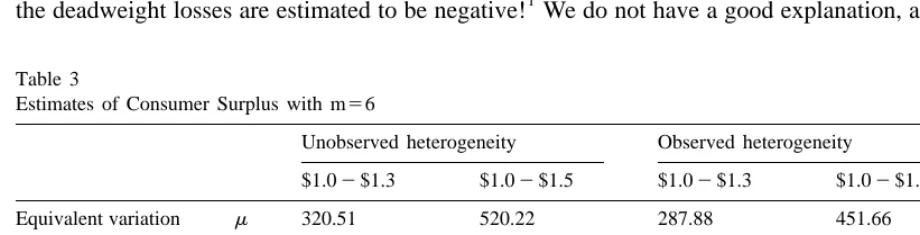
the deadweight losses are estimated to be negative! We do not have a good explanation, although one
Table 3
Estimates of Consumer Surplus with m56
Unobserved heterogeneity Observed heterogeneity
$1.02$1.3 $1.02$1.5 $1.02$1.3 $1.02$1.5
Equivalent variation m 320.51 520.22 287.88 451.66
s 149.71 261.14 82.84 130.27
Tax revenue m 299.03 515.06 261.62 390.52
s 169.48 397.80 74.98 111.93
Deadweight loss m 21.47 5.16 26.26 61.14
s 91.22 227.92 7.86 18.34
1
Table 4
Estimates of Consumer Surplus with m57
Unobserved heterogeneity Observed heterogeneity
$1.02$1.3 $1.02$1.5 $1.02$1.3 $1.02$1.5
Equivalent variation m 334.00 528.39 293.18 451.10
s 186.32 307.77 83.52 128.80
Tax revenue m 302.77 478.56 257.20 369.34
s 191.12 334.13 72.97 104.79
Deadweight loss m 31.23 49.83 35.98 81.76
s 63.67 120.97 10.55 24.01
Table 5
Estimates of Consumer Surplus with m58
Unobserved heterogeneity Observed heterogeneity $1.02$1.3 $1.02$1.5 $1.02$1.3 $1.02$1.5
Equivalent variation m 326.41 527.52 287.08 450.73
s 168.02 287.14 82.48 129.80
Tax revenue m 303.57 514.30 261.22 390.48
s 180.88 416.68 74.75 111.74
Deadweight loss m 22.84 13.22 25.85 60.25
s 88.66 234.40 7.73 18.06
possible reason may be that the standard deviation of the deadweight loss is so big that a reliable average is hard to obtain even with a large sample. This is supported by our estimates of the standard deviation of the deadweight loss. A related possibility is that our estimator does not have a fast rate of convergence: even though we have established the consistency of our procedure, we do not expect the
] Œ
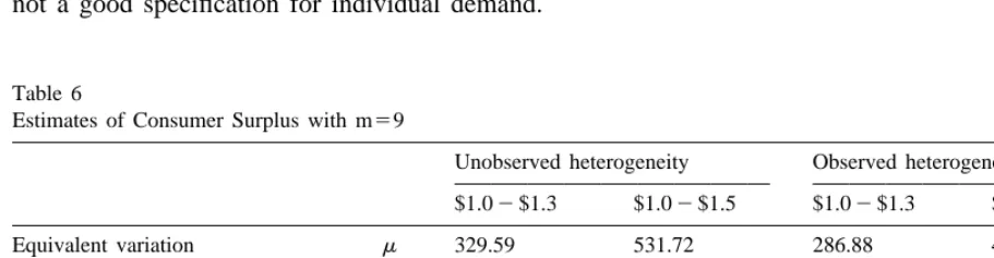
estimators to be n-consistent. Last, it may simply be the case that the log linear demand system is
not a good specification for individual demand.
Table 6
Estimates of Consumer Surplus with m59
Unobserved heterogeneity Observed heterogeneity $1.02$1.3 $1.02$1.5 $1.02$1.3 $1.02$1.5
Equivalent variation m 329.59 531.72 286.88 451.55
s 177.04 301.83 82.62 130.05
Tax revenue m 306.24 514.85 261.17 390.62
s 188.17 432.50 74.92 112.04
Deadweight loss m 23.35 16.87 25.71 59.93
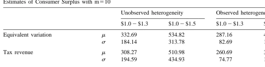
Table 7
Estimates of Consumer Surplus with m510
Unobserved heterogeneity Observed heterogeneity $1.02$1.3 $1.02$1.5 $1.02$1.3 $1.02$1.5
Equivalent variation m 332.69 534.82 287.16 450.27
s 184.14 313.78 82.69 129.95
Tax revenue m 308.27 510.98 260.69 388.68
s 194.59 434.93 74.77 111.47
Deadweight loss m 24.41 23.86 26.47 61.59
s 83.26 231.42 7.92 18.48
It is instructive to compare our estimates with Hausman and Newey’s (1995). Their equivalent variation estimates are between $278.95 and $302.75 for the price change to $1.30, and $438.01 and
2
$475.91 for the price change to $1.50. Their deadweight loss estimates are between $29.19 and $38.68, and between $45.80 and $51.05, respectively. These numbers roughly correspond to our estimates calculated under the assumption that all heterogeneity is observed. On the other hand, our equivalent variation estimates (computed under the assumption that some heterogeneity is un-observed) are between $317.46 and $332.69 for the price change to $1.30, and $513.85 and $534.83 for the price change to $1.50. This difference seems to suggest that the unobserved heterogeneity may be more important than the demand function specification. Our deadweight loss estimates for the price change to $1.30 are roughly comparable to their numbers, whereas the ones for the price change to $1.50 are not. Again, we do not very well understand why the numbers are so much different for the latter price change. Focusing on the former price change, though, we observe that most of the difference between our numbers and Hausman and Newey’s (1995) can be attributed to the tax revenue calculation.
Acknowledgements
We have benefitted from helpful comments by Joshua Angrist, Valentina Corradi, Christian Gourieroux, and the seminar participants of the University of Pennsylvania, Harvard / MIT, and CentER. We are grateful to Jerry Hausman and Whitney Newey for kindly sharing the data.
References
Beran, R., Hall, P., 1992. Estimating coefficient distributions in random coefficient regressions. Annals of Statistics 20, 1970–1984.
2
Beran, R., Millar, P., 1994. Minimum distance estimation in random coefficient regression models. Annals of Statistics 22, 1976–1992.
Hausman, J., 1981. Exact consumer’s surplus and deadweight loss. American Economic Review 71, 662–676.