Cyclical economic conditions and school attendance in Costa
Rica
Edward Funkhouser
Department of Economics, University of California, Santa Barbara, CA 93106, USA
Received 14 August 1995; accepted 22 August 1997
Abstract
In this paper, I examine the importance of declining economic conditions in school attendance decisions for house-holds with teenagers aged 12–17 in Costa Rica. I estimate a reduced-form model for school attendance that includes variables to measure household labor market integration, other household factors, teenager characteristics, regional effects and year effects. The year effects — to measure cyclical factors — show a large drop in school attendance not otherwise explained by the household variables included between the years of macroeconomic recession (1981–1983). These changes coincide with fiscal austerity imposed towards the end of 1982. In addition, household labor market characteristics and teenager characteristics are significant determinants of teenager school attendance.1998 Elsevier Science Ltd. All rights reserved.
1. Introduction
For many developing countries that have successfully implemented general primary education, the most important aspects of educational policy are now related to increases in coverage and quality at the secondary level. In most countries these policies have included changes in the compulsory schooling age, increased availability of secondary schools, increases in teacher qualifications, and the provision of better resources to existing schools. But whereas differences in school attendance at the primary level is closely related to avail-ability of educational opportunities for students of pri-mary age, for teenagers of working age, availability of educational opportunities at the secondary level is only one component of the schooling decision. In addition, changes in labor market conditions affect the allocation of time between school attendance, work, and leisure time.
Recent research on school attendance in developing countries has focused on the role of household character-istics, including income and poverty, in school enrollments (Behrman and Wolfe, 1984; Schultz, 1988;
0272-7757/98/$ - see front matter1998 Elsevier Science Ltd. All rights reserved. PII: S 0 2 7 2 - 7 7 5 7 ( 9 7 ) 0 0 0 5 3 - 8
Rosenzweig, 1990; Behrman and Deolalikar, 1991; Paes de Barros and Silva Pinto de Mendonca, 1991; Behrman et al., 1992; Deolalikar, 1992), the quality–quantity trade-off in children (Knodel and Wongsith, 1991), and differences by gender and birth order in school enrollments (Deolalikar, 1992; Parish and Willis, 1992). There has been little research on the role of cyclical economic factors in increasing the number of secondary students who do not continue their schooling. Given the importance of the world recession of the early 1980s on household incomes in the developing world, these issues may be quite important. The finding of importance of household economic variables in the school enrollment decision would have implications for educational policy during periods of economic recession. Governments con-cerned about changes in attendance should consider countercyclical policies to stimulate secondary school attendance in order to stabilize attendance levels during cyclical swings.
the developed countries on the effect of labor market conditions on school attendance has focused on intergen-erational transmission of education through parent wealth and the effects of demographic cohort size on future labor market outcomes and educational attain-ment. A common finding in the former studies is a posi-tive relationship between both household wealth and par-ent education and educational attainmpar-ent of children (Fuller et al., 1982; Margo, 1987; Haveman et al., 1991). In the latter group, several studies have shown that wages of otherwise similar workers tend to be inversely related to the size of birth cohort (Welch, 1979; Berger, 1985; Bloom et al., 1987). Studies of the effect of these wage patterns on school attendance have been less unani-mous, though most studies have tended to show that both the quantity of schooling and the amount of time required to achieve a given level of schooling increase among persons in larger birth cohorts (Wachter and Wascher, 1984; Falaris and Peters, 1992).
But since the school attendance decision depends on the labor market outcomes of both the student and other family members, the sign of changes in school attend-ance from a general decline in wages, for example, is not known a priori. Though the own-wage substitution effect from lower market wages leads to an increase in the demand for schooling, the income effect from a decline in household income could be associated with a decline in schooling demand. Therefore, aggregate evi-dence that does not reveal a strong relationship between cyclical wage changes and school attendance may be masking two opposing patterns. Other macroeconomic factors, such as changes in government spending, also affect school attendance during economic recession.
Aggregate evidence from the United States over the early 1980s does not suggest that enrollment rates were responsive to cyclical wage changes. The aggregate enrollment rate of persons aged 16 to 24 in the United States stayed constant at 30 percent over the early 1980s while real wages fell by 5.1 percent.1 Studies on the
effect of own-wage changes on school enrollments have found mixed evidence for the case of the United States. Card (1992), for example, does not find much effect of changes in the minimum wage on school enrollments while Neumark and Wascher (1995) conclude that there is an effect of the minimum wage on the skill level of teens sought by employers and — because the lower skilled teens are less likely to enroll in school — school enrollments.
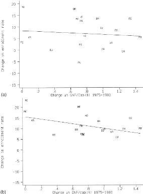
Similarly, cross-sectional evidence from the countries of Latin America, shown in Fig. 1, do not reveal a strong relationship between changes in real gross national pro-duct per capita and percentage point changes in school enrollments. In Fig. 1(A and B), the percentage change
1See U.S. Bureau of Labor Statistics (1989, Table 63).
in gross national product between 1975 and 1980 is plot-ted against changes in gross school enrollment rates at the primary and secondary levels.2 During this period,
gross national product per capita was growing in all countries except Nicaragua and Peru and school enrollment rates were increasing in most countries. Dur-ing this period of expansion there is not a statistically significant relationship between GNP per capita and enrollment rates at either the primary or secondary lev-els.
In Fig. 1(C and D), the relationship between GDP per capita and enrollments for the period 1980–1983 are shown. During these years, the mean for both economic growth and enrollment rates are lower than in the earlier period. As in the earlier period, for both primary and secondary enrollment rates, the relationship between growth in GNP per capita and change in enrollment rates is statistically insignificant.
In Fig. 1(E and F), the relationship for the period 1983–1988 — the last year in which there is data for a large sample of countries — is shown. In contrast to the earlier period, most countries experienced declines in real gross national product per capita and many also suf-fered declines in gross enrollment rates. But even during this period of contraction as well there is not a strong relationship between the magnitudes of declines in GDP per capita and school enrollments. There is a positive relationship between changes in GNP per capita and enrollment rates at the primary level and a negative relationship at the secondary level, with only the primary relationship being statistically significant. To the extent that there is a pattern in these data, it appears that changes in primary school enrollments are positively related to economic growth within a country and changes in secondary school enrollments are negatively related to economic growth.3This latter finding would indicate that
the intertemporal substitution in response to own-wage changes dominates the household income response.
In Costa Rica, though, secondary school enrollments and percentage change in GNP per capita both fell during the period 1980–1983. In Fig. 1(D), it can be seen that, of the reported countries, Costa Rica (CR) experienced the largest drop in secondary school enrollments during the period 1980–1983. Costa Rica also experienced the largest percentage drop in GNP per capita during these
2The gross school enrollment rate is school enrollment of all
students at a given level as a percentage of the number of chil-dren in the age groups that would normally be at that level. The data on gross school enrollment rates and real gross domestic product are found in Wilkie (1990).
3When controls for the initial level of GNP are included,
Fig. 1. Change in primary enrollment and secondary enrollment, respectively, (A,B) 1975–1980, (C,D) 1980–1983, (E,F) 1983– 1988, controlling for initial GNP per capita.
years. Following 1982, Costa Rica was one of the first Latin American countries to successfully implement sta-bilization policies to control inflation, the government deficit, and the external account. Since these policies accentuate effects on both the supply and demand for secondary level education, the decline in school enrollments associated with the decline in economic activity in the early 1980s make Costa Rica a particularly interesting case for the study of the effects of cyclical factors on school enrollments.
In this paper, I examine the labor market determinants of school attendance using household data in a developing country that experienced both a rapid increase in the supply of education in the 1970s and a substantial worsening in the labor market in the early 1980s. I utilize annual data for 1980–1985 in Costa Rica
to estimate a reduced-form school attendance decision model that allows estimation of both own-wage and cross-wage effects.
Costa Rica has high levels of literacy and education that resulted from social investments beginning in the last century. By the early 1980s, literacy was over 90 percent and primary education was general in both rural and urban areas. Expansion at the secondary and tertiary levels has been more recent.4But Costa Rica was also
among the countries most affected by the debt crisis and recession following the 1979 oil price shock. The period from 1980 to 1982 included a 9.4 percent drop in real GDP, an increase in inflation to 108.9 percent annual
Fig. 1. Continued.
rate in September 1982, and significant adjustment in the external sector.
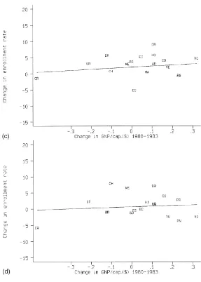
Basic patterns in wages and enrollments during the 1980s are shown in Fig. 2. The pattern in real wages of workers affiliated with the social insurance system and the mean wages reported in the annual household survey are shown in Fig. 2(A). The long-run increasing trend in real wages was broken by a large drop in real wages between 1980 and 1983 during the period of economic crisis. The real minimum wage, an alternative measure of the opportunity wage of teenagers, also fell substantially during this period (Fig. 2B).
In the next two graphs of Fig. 2, I report changes in school enrollments using school enrollment data from the educational system (Ministerio de Educacion Pub-lica, 1969, 1991) and from tabulations for attendance from the National Household Survey conducted in July
of each year from 1976 to 1992. During the period of the drop in real wages, school enrollments in grades 7– 12 fell in absolute numbers (Fig. 2C) and the proportion of children in the annual household survey aged 12–17 reporting school attendance also fell (Fig. 2D). These aggregate data do show a correlation between wages and school enrollments. I now turn to explaining these pat-terns.
2. Model
Fig. 1. Continued.
lower current income and any utility changes from time spent in school.5
Consider a household that lives for two periods. In the household are adults and children who become adults after the first period. During the first period, children may enter school, enter the workforce, or consume leis-ure while adults may not go to school. During the second period, all members of the household engage in market labor or consume leisure.
The household maximizes a utility function subject to a budget constraint, a time constraint for each member, a production function for child quality that includes years of schooling as an argument, and a market wage
determi-5More general models that incorporate family fixed effects
including permanent income such as that of Foster (1995) require longitudinal data.
nation relation. Assuming a separable utility function over time, the household problem is then:
Max
C,T,L
Σ(11d)−tU(C
t,Qj,L1t,…,Lit,…,Lnt, (1)
T1t,…,Tjt,…,Tkt;Xft,fct)
in which Ct is consumption in the household at time t,
Qjis quality of the child, Lit is leisure (family time) of
each of the n household members, Tjt is time spent in
school for each of the k children (equal to zero in the second period), Xftis observable family characteristics at
time t, andfcis community effects at time t.
Maximization of Eq. (1) is subject to four constraints. First, the budget constraint can be written:
O
t(11r)−tP ct1
O
k
PstEjt2ΣO ti
(11r)−tw
Fig. 2. (A) Real wage in social insurance and HH data, 19795100. (B) Real minimum wage, January 19795100.
2Y50
whereris the market rate of interest, Pcis the price of
the consumption good, Pst is the price of schooling, Ejt
is an indicator function for the enrollment of child j, wit
is the wage rate and Hit are the labor market hours of
individual i in the household, and Y is initial non-labor income of the household.
With borrowing and lending, the present discounted value of consumption over the lifetime of the house-hold — including consumption of schooling — is equal to the present discounted value of lifetime income and current income should matter only to the extent that it is a predictor of lifetime income. With borrowing and lending constraints, the budget constraint must hold per-iod by perper-iod and current income during the time of the attendance decision is the only income that matters.
The second constraint is the time allocation restriction for each household member:
T5Lit1EjtTit1Hit (1b)
where T is total time of individual i and Tit is time in
school of individual i. Time allocated to family time, school, and labor market activities must be equal to total time available during each period.
The third constraint is the production function for child quality that includes previous schooling, current time spent in school, potential time with other family members, observable individual characteristics, and unobservable individual characteristics.
Qj5Q(Sj, TsjtEjt,ΣLiV9j,dj) (1c)
Fig. 2. (C) Secondary enrollments. (D) Percentage of teenagers aged 12–17 in school, hh Survey.
V9is a vector of individual child factors affecting school quality, anddis unobservable quality of child j.
The last constraint is the wage determination function faced by each individual in the labor market. Own wages depend on:
wit5awt1bwtV
*
it1rstSit1buuc1uit (1d)
where V*is a vector of observable characteristics, r
s is
the return to schooling, anducis a vector of conditions
in the local labor market.6
The first order-condition for time spent in school states
6The basic administrative district in Costa Rica is called a
canton. The data forucare calculated separately for urban and
rural areas within each canton.
that the marginal benefit in child quality plus direct util-ity gained from an increase in time spent from school is equal to the marginal cost in fees plus the marginal opportunity cost:
dU dQj
dqj
dsj
dsj
dtsj
1du dtj
2l{Ps1wjt2(1 (2)
1i)−1r
s,t11}50
The demand for time devoted to school, Tsj can be
written in reduced form as:
Tsj5Tj(Pc, Ps, wL, Y, rs, Xf, NfV,fc,dj) (3)
in which the vector V now includes V9and V*and the
non-arbitrary fashion, within the household, time allocation decisions of adults are made prior to the time allocation decision of children. With a sequential decision process in which adults make labor market decisions before teen-agers make their time allocation decisions, teenteen-agers condition their work and school decision on the actual labor market outcomes of adults. In this case, pooling data across years and assuming that each teenager makes the time allocation decision independently of other teen-agers in the household and the price of consumption goods can be normalized to one, a first-order approxi-mation of Eq. (3) can be written:
Tsj5a 1 bswˆj5
O
in which the predicted wage, wj, is the opportunity cost
of attending the next year of school for teenager j,ftis
vector of year effects, andej is an error that includes
unobservable individual effects, dj, and any random
effects. Tsjis the indicator function for school attendance
of child j:
E51 if Tsj > 0 (5)
E50 if Tsj #0
The estimation procedure involves four steps. First, mean wages within each canton and urban cell, con-trolling for other factors, are calculated for each year from the sample of all workers to proxy for opportunities in the local labor market. The second step is the calcu-lation of predicted wages for each teenager using Eq. (1d) estimated separately by year. The predicted wages for individual j at time t estimated from the sample of working teenagers is then applied to all teenagers aged 12–17 as a measure of Ps. This equation is identified by
the labor market opportunities variable. Third, the return to the next year of education is calculated from the esti-mation of a wage equation for all workers in the same year as the school attendance decision is made is used as a proxy for the future income differential resulting from the investment in an additional year of education. The fourth step is the estimation of the reduced form attendance equation, Eq. (4).
3. Data
In this study, I utilize the Encuesta Nacional de Hogares, Empleo, and Desempleo conducted by the Direccion General de Estadistica y Censos (DIGESTYC) in Costa Rica. The survey was conducted with an
inde-pendent sample in July of each year from 1980 to 1983 and in 19857and includes demographic and labor market
information for household members aged 12 and above.8
Each person is asked whether they currently attend school and the last grade attended. There are 22 798 chil-dren aged 12–17 in the 5 years of the survey from 1980 to 1983 and 1985. 56.4 percent of all children report that they attend school. Of those who attend school, 2.66 per-centage points report that they also work. And of the 43.6 percent who do not attend school, 19.1 percentage points report their main activity as working.
Information on other household members — including employment status of the head of the household, the number of other working household members, the num-ber of non-working household memnum-bers, numnum-ber of chil-dren under 12, income of head,9income of next highest
earner,10 and other income — was obtained by
recon-structing households. These data were then merged with the individual level data for teenagers.
The opportunity wage of each teenager is predicted from a wage equation using the sample of working teena-gers. The identifying variables in this equation are the mean wage and unemployment rate of all workers in the local labor market (calculated separately for the urban and rural areas in each canton) in which the teenager resides. The regressions from which these predicted values are calculated are shown in Appendix A. With the exception of the equation for 1981, the pattern in teenage wages is a positive relationship between teenage wages and each of mean wages in the canton (calculated from all workers), experience, and education. Girls earn substantially less than males in all years. And there is no clear pattern in relative wages of teenagers in urban areas once education and mean wages have been con-trolled for.
The return to education for each additional year of education was estimated utilizing the complete sample for each year and including a dummy variable for each
7The survey has been conducted from 1976 to 1992. In
addition, there are also March and November surveys which do not include information on education. The survey was not conducted in July 1984 in order to conduct a Census at that time. There are two reasons that the period 1980–1985 is included in this study. First, these are the years before and dur-ing the economic recession and any effect on school enrollments should be observed during these years. Second, the survey format is different in surrounding years.
8Before 1980, earnings information is available only for
wage and salary workers. Starting in 1980, earnings questions were asked of all workers.
9Nominal values were deflated by the July value of the
con-sumer price index for the San Jose metropolitan area (Banco Central de Costa Rica, 1986).
10Highest non-head earner is used because relationship to
year of education. The returns estimated using this pro-cedure are shown in Appendix B. These values were matched by calendar year to the next year of education for each teenager in the survey.11
3.1. School attendance patterns of teenagers aged 12– 17
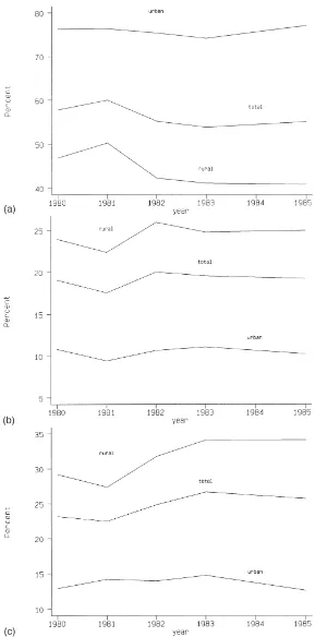
School attendance patterns of teenagers aged 12–17 using adjusted sample weights12
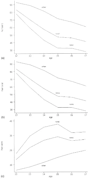
are shown by year in Fig. 3 and by age in Fig. 4. In each figure, Panel A includes the percentage of teenagers in school, Panel B includes the percentage of teenagers only working, and Panel C includes the percentage of teenagers neither in school nor working. The three lines in the figures report these percentages for all teenagers, teenagers in rural areas, and teenagers in urban areas. As can be seen in all of the graphs, the proportion of teenagers aged 12– 17 attending school is much lower in rural areas than in urban areas. And the proportion that reports neither school attendance nor work is much higher in rural areas than in urban areas.
The overall pattern by year shows a slight drop in the percentage attending school (Fig. 3A), a slight increase in the percentage only working (Fig. 3B), and a more gradual increase in the percentage that neither are in school nor work (Fig. 3C) over the period of economic recession (1981–1983). Nearly all of the change, though, occurred in rural areas. This initial evidence indicates that the effect of cyclical conditions on school attendance differed between rural and urban areas.
The patterns by age also reveal differences between rural and urban areas in the activities of teenagers. There is a large drop in the proportion attending school between the ages of 12 and 15 in rural areas (from 75.9 percent to 30.6 percent) compared to a more gradual decline over these age groups in urban areas (from 91.6 percent for those 12 years old to 69.7 percent for those 15 years old).
In Fig. 4, school and work patterns are shown by age of the child. 81.5 percent of children age 12 are reported to be attending school only. By age 17, only 35.8 percent are only attending school. The drop-off in attendance rates is quite large immediately following the completion of primary education between the ages of 12 and 15. Approximately half of the decline corresponds to an increase in those who work and half corresponds to those who neither work nor attend school. Above 15 years of
11An alternative approach would be for children to have
expectations about the return to each year of education at the time they are expected to be in the labor market.
12In addition, weights were calculated that reflect the
popu-lation reported in the 1973 and 1984 Censuses in place of the reported weights in the data files.
age, all declines in attendance correspond to increases in those who only work. There is little change in the pro-portion who attend school and report working as age increases.
Fig. 3 showed a slight drop in the proportion of teena-gers aged 12–17 that were attending school at the time of the survey. The permanence of the decline in school attendance rates during the years of economic recession can be examined by following age cohorts over time. With the assumption that secondary schooling (11 years) is completed by age 23, final educational years of school-ing indicates whether attendance declines reflect either lower final attainment or a longer period required to attain a given target level of education.
In Fig. 5, the proportion of each age cohort (defined by age in 1980 along the horizontal axis) with at least 11 years of education is shown at age 18 (bottom line), age 19, ages 20–22, and ages 23–25 (top line). In this figure, I include grade completion information from all of the household surveys from 1976 to 1992. For example, 25 percent of the cohort that was born in 1966 and was 14 years old in 1980 had finished at least 11 years of school four years later in 1984. Reading upwards, 27 percent had 11 years of education in 1985 at 19 years old and approximately 30 percent had 11 years by the ages 20–25. The difference between any two lines indicates the proportion of a birth cohort that attained 11 years of education between the indicated ages. Because cohorts that were born earlier were older in 1980, the general increase in educational attainment of sequential cohorts is seen from the increase in the proportion of each cohort that has a secondary education at each age level as the figure moves from right to left. The age groups who were obtaining their secondary education during the years of economic crisis (1980– 1982) were those aged 12–17 in 1980. Two patterns are of interest. First, at all ages, there is a leveling off in the proportion that had attained 11 years of schooling for birth cohorts that were younger than 18 in 1980, with the final rate of each cohort between 29 and 33 percent. For the youngest cohorts during the recession and those that became teenagers after the recession (age less than 12 in 1980), the secondary completion rates at age 20– 22 are lower than earlier cohorts. This corresponds to the decreased enrollments seen in Fig. 2(C) and (D). Second, secondary education completion occurred earlier for birth cohorts that were under 14 in 1980. These cohorts were entering secondary school age during or after the economic crisis.
3.2. Characteristics by type of activity
Fig. 5. Percentage of birth cohort with 111years school.
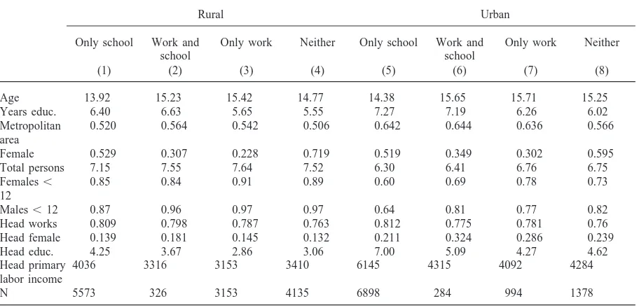
Table 1
Characteristics of teenagers aged 12–17 by school and work status
Rural Urban
Only school Work and Only work Neither Only school Work and Only work Neither
school school
(1) (2) (3) (4) (5) (6) (7) (8)
Age 13.92 15.23 15.42 14.77 14.38 15.65 15.71 15.25
Years educ. 6.40 6.63 5.65 5.55 7.27 7.19 6.26 6.02
Metropolitan 0.520 0.564 0.542 0.506 0.642 0.644 0.636 0.566
area
Female 0.529 0.307 0.228 0.719 0.519 0.349 0.302 0.595
Total persons 7.15 7.55 7.64 7.52 6.30 6.41 6.76 6.75
Females, 0.85 0.84 0.91 0.89 0.60 0.69 0.78 0.73
12
Males,12 0.87 0.96 0.97 0.97 0.64 0.81 0.77 0.82
Head works 0.809 0.798 0.787 0.763 0.812 0.775 0.781 0.76
Head female 0.139 0.181 0.145 0.132 0.211 0.324 0.286 0.239
Head educ. 4.25 3.67 2.86 3.06 7.00 5.09 4.27 4.62
Head primary 4036 3316 3153 3410 6145 4315 4092 4284
labor income
N 5573 326 3153 4135 6898 284 994 1378
Source: Tabulations by author.
There are several patterns that are common to both rural and urban areas. First, those who work tend to be older and to have less education than those who were attending school at the time of the survey. Second, though approxi-mately half of those enrolled in school are female, females are much less likely to be working than are males; 72 percent of the teenagers that neither attend school nor work in rural areas and 60 percent in urban areas are female. Third, the education of the head of the household is positively correlated with school attendance
by teenagers, though this may reflect household compo-sition rather than parent’s education. And lastly, employ-ment rates and mean income of the head of households in which the teenager attends school are higher than those in which teenagers work.
in which the head has higher mean education, and live in households with higher income.
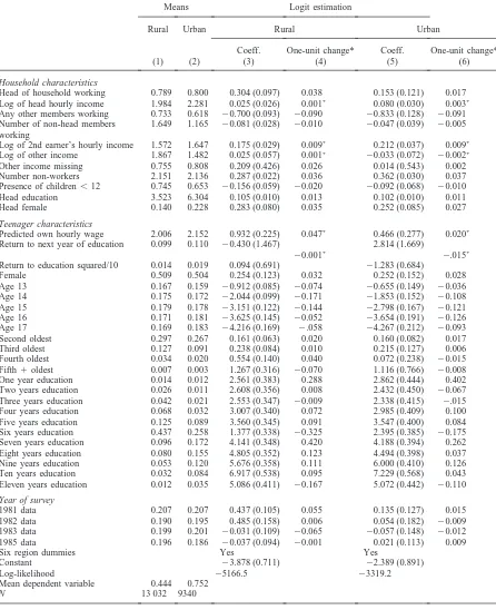
4. Estimation results
In this section, I estimate the determinants of school attendance in Eq. (5) using pooled data for 1980–1985. These results are reported in Table 2. In the first two columns, means of each variable are reported for rural and urban areas.13In columns (3) and (5) of Table 2, the
results of the logit estimation for school attendance are shown for rural and urban areas. The marginal prob-abilities — calculated holding other characteristics fixed to actual values for each individual — are shown in Col-umns (4) and (6).
4.1. Household characteristics
The first set of variables describe household character-istics. These variables are organized into three groups. The first group — head employed, logarithm of head hourly income, presence of other workers, number of other workers, logarithm of second earner hourly income, presence of other income, logarithm of other income — describes the employment and earnings out-comes of household members in which the teenager resides. The second group — number of non-workers and presence of children under 12 — describes the types of non-workers that are in the household. The third group describes two other characteristics of the head of the household: education of the head and a dummy variable for female head.
Taken together, the coefficients on the household labor market variables present an interesting picture of the relationship between work and school for teenagers in Costa Rica. It is useful to note that the magnitude of the effects seen in columns (4) and (6) are quite similar in rural and urban areas.
Better labor market outcomes of the head are associa-ted with a higher probability of school attendance, though the pattern is weak. For employment, the increase in attendance associated with the head being employed is 3.8 percentage points in rural areas and 1.7 percentage points in urban areas. Of more statistical importance is the pattern between school attendance and the labor mar-ket outcomes of household members other than the head. Both the presence and number of non-head members
13For logarithm of head hourly wage, the logarithm of the
next earner’s hourly wage, and logarithm of non-wage income, zero was assigned for zero values in levels and separate vari-ables for head working, number of head workers, and non-wage income missing were included. For this reason, the mean value of each of the logarithm variables includes zero values.
who are working is associated with lower probability of current school attendance and the magnitude of the mar-ginal changes are larger than those found for the head. Given the number of non-heads working, though, a higher hourly wage earned by the second earner — and higher income in the household — is associated with a higher probability of school attendance. One possibility for explaining the former pattern is that the costs of search in the labor market are reduced with more house-hold members in the labor market.
The presence of non-working members in the house-hold are also important. The presence of other non-work-ing adults in the household is associated with higher school attendance — by 3.6 percentage points in rural areas and 3.7 percentage points in urban areas. In con-trast, the presence of younger children is a deterrent to school attendance — by 2.0 percentage points in rural areas and 1.0 percentage points in urban areas.
4.2. Teenager characteristics
The next rows of Table 2 report the coefficients on the variables related to the teenager characteristics, with two labor market variables (predicted own-wage and return to the next year of education) and several demo-graphic characteristics (female, age, birth order, and education). The effect of the predicted own-wage effect is positive and significant, with a 50 percent increase associated with a higher probability of school attendance by 4.7 percentage points in rural areas and 2.0 percentage points in urban areas. These coefficients are not consist-ent with the predicted wage measuring the opportunity cost of school attendance and may reflect lifetime wealth as a proxy for future income.14The effect of the return
to education is small and less conclusive. The net effect of a 50 percent increase in education is zero in rural areas and negative in urban areas.15
Demographic factors are important determinants of school attendance. Females are approximately three per-centage points more likely to attend school in both rural and rural areas. There are large effects of age on school attendance, even controlling for completed education. Each of the entries in the column for marginal prob-abilities measures the change in probability of attendance for teenagers of the given age compared with otherwise
14When the age dummy variables are not included, the
coef-ficient on the predicted wage is negative and significant. Since the variation in predicted wage comes from regional labor mar-ket characteristics, those areas with worse labor marmar-ket out-comes have lower attendance rates.
15With the inclusion of dummy variables for each year of
Table 2
Determinants of school attendance 1980–1985
Means Logit estimation
Rural Urban Rural Urban
Coeff. One-unit change* Coeff. One-unit change*
(1) (2) (3) (4) (5) (6)
Household characteristics
Head of household working 0.789 0.800 0.304 (0.097) 0.038 0.153 (0.121) 0.017 Log of head hourly income 1.984 2.281 0.025 (0.026) 0.001* 0.080 (0.030) 0.003*
Any other members working 0.733 0.618 20.700 (0.093) 20.090 20.833 (0.128) 20.091 Number of non-head members 1.649 1.165 20.081 (0.028) 20.010 20.047 (0.039) 20.005 working
Log of 2nd earner’s hourly income 1.572 1.647 0.175 (0.029) 0.009* 0.212 (0.037) 0.009*
Log of other income 1.867 1.482 0.025 (0.057) 0.001* 20.033 (0.072) 20.002*
Other income missing 0.755 0.808 0.209 (0.426) 0.026 0.014 (0.543) 0.002 Number non-workers 2.151 2.136 0.287 (0.022) 0.036 0.362 (0.030) 0.037 Presence of children,12 0.745 0.653 20.156 (0.059) 20.020 20.092 (0.068) 20.010
Head education 3.523 6.304 0.105 (0.010) 0.013 0.102 (0.010) 0.011
Head female 0.140 0.228 0.283 (0.080) 0.035 0.252 (0.085) 0.027
Teenager characteristics
Predicted own hourly wage 2.006 2.152 0.932 (0.225) 0.047* 0.466 (0.277) 0.020*
Return to next year of education 0.099 0.110 20.430 (1.467) 2.814 (1.669)
20.001* 2.015*
Return to education squared/10 0.014 0.019 0.094 (0.691) 21.283 (0.684)
Female 0.509 0.504 0.254 (0.123) 0.032 0.252 (0.152) 0.028
Age 13 0.167 0.159 20.912 (0.085) 20.074 20.655 (0.149) 20.036
Age 14 0.175 0.172 22.044 (0.099) 20.171 21.853 (0.152) 20.108
Age 15 0.179 0.178 23.151 (0.122) 20.144 22.798 (0.167) 20.121
Age 16 0.171 0.181 23.625 (0.145) 20.052 23.654 (0.191) 20.126
Age 17 0.169 0.183 24.216 (0.169) 2.058 24.267 (0.212) 20.093
Second oldest 0.297 0.267 0.161 (0.063) 0.020 0.160 (0.082) 0.017
Third oldest 0.127 0.091 0.238 (0.084) 0.010 0.215 (0.127) 0.006
Fourth oldest 0.034 0.020 0.554 (0.140) 0.040 0.072 (0.238) 20.015
Fifth1oldest 0.007 0.003 1.267 (0.316) 20.070 1.116 (0.766) 20.008
One year education 0.014 0.012 2.561 (0.383) 0.288 2.862 (0.444) 0.402 Two years education 0.026 0.011 2.608 (0.356) 0.008 2.432 (0.450) 20.067 Three years education 0.042 0.021 2.553 (0.347) 20.009 2.338 (0.415) 2.015 Four years education 0.068 0.032 3.007 (0.340) 0.072 2.985 (0.409) 0.100 Five years education 0.125 0.089 3.560 (0.345) 0.091 3.547 (0.400) 0.084 Six years education 0.437 0.258 1.377 (0.338) 20.325 2.395 (0.385) 20.175 Seven years education 0.096 0.172 4.141 (0.348) 0.420 4.188 (0.394) 0.262 Eight years education 0.080 0.155 4.805 (0.352) 0.123 4.494 (0.398) 0.037 Nine years education 0.053 0.120 5.676 (0.358) 0.111 6.000 (0.410) 0.126 Ten years education 0.032 0.084 6.917 (0.538) 0.095 7.229 (0.568) 0.043 Eleven years education 0.012 0.035 5.086 (0.411) 20.167 5.072 (0.442) 20.110 Year of survey
1981 data 0.207 0.207 0.437 (0.105) 0.055 0.135 (0.127) 0.015
1982 data 0.190 0.195 0.485 (0.158) 0.006 0.054 (0.182) 20.009
1983 data 0.199 0.201 20.031 (0.109) 20.065 20.057 (0.148) 20.012
1985 data 0.196 0.186 20.037 (0.094) 20.001 0.021 (0.113) 0.009
Six region dummies Yes Yes
Constant 23.878 (0.711) 22.389 (0.891)
Log-likelihood 25166.5 23319.2
Mean dependent variable 0.444 0.752
N 13 032 9340
Note: One-unit changes are calculated by increasing indicated variable by unit while holding all other variables constant at their actual values. For sequential dummy variables (i.e. age, years of education, year), changes are between categories. Changes are 50 percent increases for variables indicated by an asterisk.
similar teenagers one year younger. Each of these entries is negative, large, and statistically significant.
In the next rows of the table, the birth order of the teenager within the group of teenagers aged 12–17 within the household is shown.16For example, 29.7
per-cent of the teenagers in the sample for rural areas had an older sibling aged 12–17. These teenagers are 2.0 per-centage points more likely to attend school than their older siblings. Continuing down the column, third-oldest teenagers in rural areas are 1.0 percentage points more likely to attend school than the second-oldest and 3.0 percentage points more likely than the oldest sibling. The data show that younger teenagers are more likely to attend school than their older school age siblings.
The next rows of Table 2 show the effect of previous education on current school attendance. These coef-ficients show that teenagers in the sample tended to com-plete schooling in the curriculum cycles of the edu-cational system in Costa Rica (1–6, 7–11).17There are
large drops in the probabilities of current attendance for those who had completed zero years of education, six years of education, and eleven years of education.
4.3. Year effects
In Fig. 3, the pattern over the years of recession showed a drop in school attendance in rural areas and little change in urban areas. The final coefficients in Table 2 show these year effects in school attendance with controls for the other variables included. Though not entirely attributable to regional or macroeconomic con-ditions because there may be time-varying household characteristics not otherwise included, these coefficients provide a rough indicator of the importance of factors outside the household in explaining school attendance.
The results indicate that there is not much variation in school attendance that is explained by changing con-ditions over the early 1980s in urban areas, but that these factors are important in explaining the drop in school attendance in rural areas. Though the general pattern for rural areas in the table is similar to that in the previous figure — there is a one-time drop in attendance rates without much rebound — the timing of the change is one-year later with controls than that without controls. In rural areas, there is a 7.1 percentage point drop in attendance rates observed between 1981 and 1982 in Fig. 1. In contrast, between these two years there is no change in the year effect with controls in Table 2. The drop in the year effect occurs instead between 1982 and 1983.
16This is not necessarily the true birth order of the teenager
since siblings older than 17 or siblings that do not live in the household are not counted.
17Note that the marginal probabilities are calculated relative
to one fewer year of education.
This pattern is explained by changes in the mean values of other explanatory variables in directions associated with lower school attendance between 1981 and 1982 and in directions associated with higher school attend-ance between 1982 and 1982. In particular, a worsening of the predicted own wage and the changing age distri-bution within the category of teenagers between 1981 and 1982 were the largest contributors to lower attend-ance between these years.
Expressed in terms of changes in the standardized lat-ent variable in the attendance decision, changes in the predicted own wage contribute 2 0.302 compared to 0.048 for the year effect between 1981 and 1982. Other teenager characteristics, mainly age, contribute20.180; household economic characteristics contribute20.061; and other household characteristics contribute20.041. Between 1982 and 1983 the contribution of all of these categories is towards higher school attendance. The year effect, though, is a reduction of 0.516 in the latent vari-able — or 6.5 percentage points in attendance rates — between 1982 and 1983.18
5. Extensions
In this section, I examine several extensions of the results presented in Section 3. The results of these exten-sions are shown in Table 3 for the rural sample in Panel A and the urban sample in Panel B. Though only a subset are reported, all of the control variables from Table 2 are included in each specification.
First, separate estimates of the determinants of school attendance are presented for males and females in col-umns (1) and (2). Second, the possibility that the relationship between previous education on current attendance is masking other relationships is examined with two approaches. The first is designed to counteract the low attendance of older teenagers with low previous education not captured by age and education dummy variables separately. In column (3), interactions for each age and years of education combination are included. The second approach, in Column (4) is the restriction of the sample to households with only one teenager and is designed to counteract the natural relation between second teenagers and lower levels of education. In col-umn (5), controls for geographic fixed effects at the can-ton level are included. Finally, in column (6), controls for selectivity in the employment decision are included in the calculation of the predicted values of the opport-unity wage of teenagers.
The patterns in the determination of school attendance in these data are quite robust to specification and sample.
18The lag in the macroeconomic effect suggests a role for
Table 3 Extensions
Male Female Age-education Single teenager Canton fixed Heckman corr. inter. households effects
(1) (2) (3) (4) (5) (6)
Panel A: Rural
Predicted own 1.069 (0.268) 0.324 (0.244) 1.121 (0.230) 0.613 (0.446) 0.285 (0.248) 0.121 (0.076) hourly wage
Household characteristics
Head of 0.500 (0.143) 0.164 (0.134) 0.296 (0.099) 0.179 (0.195) 0.287 (0.099) 0.299 (0.097) household
working
Log of head 0.010 (0.040) 0.029 (0.036) 0.023 (0.027) 0.077 (0.053) 0.025 (0.027) 0.031 (0.026) hourly income
Any other 21.055 (0.138) 20.414 (0.129) 20.709 (0.095) 20.890 (0.195) 20.662 (0.095) 20.711 (0.093) members working
Number of non- 20.114 (0.040) 20.076 (0.039) 20.091 (0.028) 20.030 (0.076) 20.051 (0.029) 20.082 (0.028) head members
working
Log of 2nd 0.154 (0.041) 0.175 (0.041) 0.177 (0.029) 0.288 (0.060) 0.132 (0.030) 0.181 (0.029) earner’s hourly
income
Log of other 0.144 (0.084) 20.058 (0.077) 0.035 (0.057) 20.012 (0.145) 20.008 (0.058) 0.031 (0.057) income
Other income 1.071 (0.627) 20.367 (0.583) 0.284 (0.432) 0.205 (1.113) 20.044 (0.438) 0.269 (0.426) missing
Number of non- 0.363 (0.033) 0.209 (0.031) 0.286 (0.022) 0.342 (0.052) 0.296 (0.023) 0.288 (0.022) workers
Presence of 20.251 (0.087) 20.061 (0.080) 20.160 (0.059) 0.047 (0.112) 20.146 (0.060) 20.158 (0.059) children,12
Head education 0.093 (0.015) 0.108 (0.013) 0.107 (0.010) 0.104 (0.019) 0.094 (0.010) 0.108 (0.010) Head female 0.331 (0.119) 0.264 (0.109) 0.278 (0.081) 0.347 (0.150) 0.197 (0.082) 0.289 (0.080) Year:
1981 data 0.408 (0.144) 0.324 (0.134) 0.488 (0.108) 0.360 (0.215) 0.288 (0.110) 20.107 (0.198) 1982 data 0.450 (0.204) 0.197 (0.183) 0.600 (0.162) 0.438 (0.317) 0.121 (0.172) 20.035 (0.085) 1983 data 20.102 (0.137) 20.213 (0.142) 0.028 (0.111) 20.003 (0.216) 20.206 (0.116) 20.405 (0.092) 1985 data 20.162 (0.129) 20.076 (0.128) 20.005 (0.095) 20.029 (0.186) 20.147 (0.098) 20.436 (0.168)
-Log likelihood 2 361.6 2 766.3 5 097.2 1 284.5 5 016.5 5 173.8
N 6 398 6 634 12 961 3 104 13 032 13 032
Panel B: Urban
Predicted own 0.772 (0.337) 20.021 (0.317) 0.452 (0.283) 0.749 (0.496) 20.030 (0.309) 20.020 (0.099) hourly wage
Household characteristics
Head of 0.324 (0.176) 20.022 (0.167) 0.151 (0.122) 20.106 (0.205) 0.135 (0.122) 0.159 (0.121) household
working
Log of head 0.091 (0.045) 0.076 (0.041) 0.077 (0.031) 0.146 (0.053) 0.085 (0.031) 0.081 (0.030) hourly income
Any other 21.156 (0.185) 20.611 (0.180) 20.829 (0.129) 20.519 (0.227) 20.849 (0.129) 20.841 (0.128) members working
Number of non- 20.074 (0.054) 20.005 (0.059) 20.043 (0.040) 20.029 (0.079) 20.039 (0.040) 20.049 (0.039) head members
Table 3 Extensions
Male Female Age-education Single teenager Canton fixed Heckman corr. inter. households effects
(1) (2) (3) (4) (5) (6)
Log of 2nd 0.247 (0.051) 0.179 (0.053) 0.205 (0.037) 0.167 (0.067) 0.209 (0.037) 0.216 (0.037) earner’s hourly
income
Log of other 20.084 (0.096) 0.009 (0.109) 20.035 (0.072) 0.031 (0.150) 20.037 (0.073) 20.032 (0.072) income
Other income 20.201 (0.730) 0.176 (0.821) 20.016 (0.547) 0.542 (1.175) 20.005 (0.554) 0.028 (0.543) missing
Number of non- 0.395 (0.042) 0.315 (0.042) 0.359 (0.030) 0.420 (0.054) 0.356 (0.030) 0.363 (0.030) workers
Presence of 20.168 (0.098) 20.024 (0.095) 20.082 (0.069) 20.100 (0.118) 20.090 (0.069) 20.094 (0.068) children,12
Head education 0.101 (0.014) 0.107 (0.014) 0.101 (0.010) 0.115 (0.017) 0.095 (0.010) 0.103 (0.010) Head female 0.210 (0.123) 0.319 (0.119) 0.258 (0.086) 0.400 (0.142) 0.232 (0.086) 0.256 (0.085) Year:
1981 data 0.158 (0.173) 0.058 (0.174) 0.142 (0.128) 0.297 (0.241) 0.014 (0.131) 20.081 (0.267) 1982 data 0.250 (0.236) 20.219 (0.221) 0.047 (0.185) 0.125 (0.326) 20.212 (0.197) 20.208 (0.111) 1983 data 0.119 (0.182) 20.315 (0.201) 20.056 (0.151) 0.093 (0.265) 20.254 (0.160) 20.230 (0.113) 1985 data 0.136 (0.157) 20.152 (0.164) 0.034 (0.115) 0.101 (0.197) 20.037 (0.117) 0.004 (0.223)
-Log likelihood 1 606.4 1 690.3 3 282.0 1 100.9 3 286.8 3 320.6
N 4 634 4 694 9 340 3 296 9 340 9 340
The main patterns are similar to those seen in Table 2. There are several findings that are common to all of these extensions. First, the presence of working household members other than the head is negatively related to school attendance. Second, the income of the second earner is positively related to school attendance. Third, the number of non-working persons age 18 and above in the household is positively related to attendance. Fourth, the education of the household head is positively related to school attendance. And fifth, teenagers in female-headed households are more likely to be enrolled in school than other teenagers.19 Sixth, the return to
edu-cation is not significantly related to school attendance. In addition, these extensions confirm differences between rural and urban areas seen in Table 2. First, employment of the household head is positively related to school attendance in rural areas and has little relation-ship in urban areas. Second, the presence of children under 12 in the household is negatively related to school attendance in rural areas and has little relationship in urban areas. Third, hourly income of the head of the household is not related to school attendance in rural areas and is positively related to school attendance in urban areas.
In columns (1) and (2), separate logit estimation was conducted for the sample of males and the sample of females. In the comparison of the two columns in each panel, the main finding is the positive relationship between predicted own hourly wage and male school
attendance while the relationship is insignificant for females. Somewhat surprisingly, the presence of children less than 12 in the household is significantly negatively related to school attendance for males, but not for females.
To allow for the possibility that teenagers are unlikely to return to school once they have missed a year, I allow for separate intercepts for each completed year of school interacted with age in column (3). In this and subsequent columns, the sample includes both males and females. The inclusion of these interactions results in little change in the estimated coefficients for all variables. Similar results are obtained when the sample is restricted to teen-agers that are within one year of the appropriate com-pleted years of education for the teenager’s age. As an additional test to verify that a relationship between age and attendance based on completed years of schooling has not been imposed, I restrict the sample to households in which only one teenager is reported in column (4). Again, there is little change in any of the coefficients on the household variables.20
In column (5), I allow more detailed controls for
geo-19Characteristics of the head may reflect household
compo-sition since the head does not have to be parent of the child.
20The one exception is in the effect of children under 12 in
graphic fixed effects by including dummy variables at the level of the canton. With the inclusion of these dummy variables, all variables should be interpreted as deviations from canton means. The main finding from this column is unsurprising result that the variable that is calculated at the canton level (predicted own wage) has less explanatory power when canton fixed effects are included. Otherwise, it is not the case that there is bias from unobserved geographic characteristics at the can-ton level.
As a final extension, I estimate the hourly wage func-tions of Eq. (1d) with a correction for self-selection using Heckman’s two-stage approach in column (6) of each panel. With the exception of the coefficient (and standard error) on this variable, there is little change in the esti-mated coefficients on the household variables once this correction is included.
As in the previous section, the coefficients on the year dummy variables indicate the effect of macroeconomic factors on school attendance. These coefficients do differ by specification and indicate that the overall patterns over time mask opposing tendencies for males and females. In both urban and rural areas, the drop in year effects between 1981 and 1982 in the raw data is seen also in the regressions for females (column 2). In con-trast, there is no drop for males between 1981 and 1982 and the drop in year effects between 1982 and 1983 seen in the aggregate regressions of Table 2 is seen in the regressions for males (column 1). In the remaining col-umns, the pattern in rural areas is similar to that pre-viously seen in Table 2 — with a drop in attendance between 1982 and 1983. In urban areas, columns (3)–(6) provide additional evidence that there was a drop in school attendance controlling for other factors between 1981 and 1982 that had been recovered by 1985.
6. Concluding remarks
In this paper, I have examined the importance of econ-omic conditions and household school attendance decisions for Costa Rica. There are three main findings. First, school attendance is positively related to the income and negatively related to the employment of other household members. The magnitude of many of these labor market effects is small, however. In addition, attendance is negatively related to the presence of chil-dren under twelve, positively related to the presence of a female head, and positively related to education of the head of the household.
Second, there is a positive relationship between the predicted wage of the teenager and school attendance that is not consistent with the idea that a higher opport-unity cost is associated with lower attendance. Because there was a large reduction in the level of the predicted wage between 1981 and 1982, a large part of the
reduction in school attendance observed over these years is attributable to the change in this variable. Age and previous education of the teenager are also important determinants of current school attendance.
Third, cyclical economic factors played a large role in the drop in school attendance in Costa Rica over the 1980s. The year effects show a drop in school attendance not otherwise explained by the household variables included between the years of macroeconomic recession (1981–1983). These changes coincide with fiscal aus-terity imposed towards the end of 1982.
The main policy implication of these findings con-cerns the effect that changes in current school attendance have on final education completion levels. In Fig. 3, it was seen that the most recent teenage cohorts have lower rates of completion of secondary than those that attended school immediately prior to the economic recession. To the extent that macroeconomic conditions affected these rates — as reflected in the year effects in the regressions — governments may consider policies to promote school attendance to offset these changes.
Acknowledgements
This paper would not have been possible without the financial assistance of the Social Science Research Council and the Academic Senate of the University of California. In addition, I have benefitted greatly from the assistance of Virginia Rodriguez, Maria Marta Baenz, and Rafael Espinosa at the Direccion General de Estadis-tica y Censos in San Jose and the comments of two anonymous referees.
Appendix A
Log wage equations used to predict opportunity wage of teenagers aged 12–17
1980 1981 1982 1983 1985
(1) (2) (3) (4) (5)
Mean 0.499 0.063 0.309 0.473 0.277
wage in canton
(0.102) (0.114) (0.117) (0.122) (0.140)
Unem- 2 2 0.241 2 1.286
ployment 0.241 0.392 0.125
rate
(0.482) (0.553) (0.509) (0.520) (0.701)
Years 0.150 0.114 0.149 0.138 0.157
of education
Years 0.034 0.108 0.110 0.055 0.112 of
experience
(0.031) (0.035) (0.030) (0.037) (0.043)
Experience0.008 2 0.002 0.008 0.001
squared 0.001
(0.003) (0.004) (0.003) (0.004) (0.005)
Female 2 2 2 2 2
0.460 0.452 0.441 0.573 0.567
(0.045) (0.053) (0.049) (0.053) (0.051)
Urban 2 0.100 2 2 2
0.170 0.073 0.145 0.036
(0.062) (0.072) (0.075) (0.068) (0.074)
Region Yes Yes Yes Yes Yes
dummies
Constant 2 1.146 2 2 0.263
0.066 0.152 0.160
(0.346) (0.384) (0.345) (0.401) (0.472)
R- 0.222 0.155 0.237 0.214 0.257
squared
N 787 687 702 691 629
Appendix B
Returns to next year of education
Return to next year of education
Past 1980 1981 1982 1983 1985
(1) (2) (3) (4) (5)
0 0.052 0.048 0.008 0.057 2
0.019
1 0.056 0.055 0.071 0.018 0.076
2 0.025 0.065 0.014 0.010 0.033
3 0.118 0.068 2 0.016 0.042
0.007
4 2 2 0.093 0.042 0.049
0.004 0.028
5 0.166 0.166 0.121 0.105 0.092
6 0.126 0.034 0.154 0.111 0.087
7 0.080 0.170 0.081 0.096 0.096
8 0.107 0.155 0.133 0.082 0.078
9 0.081 2 0.046 2 2
0.060 0.016 0.005
10 0.280 0.381 0.252 0.326 0.316
11 0.193 0.214 0.182 0.236 0.027
Note: Returns are calculated from log wage equations estimated with the complete sample for each year with dummy variables for each year of education, potential
labor market experience, experience squared, urban status, female, and region dummy variables.
References
Banco Central de Costa Rica (1986) Estadisticas 1950–1985. October. Division Economica, San Jose.
Behrman, J., Deolalikar, A., 1991. School repetition, dropouts, and the returns to schooling: the case of Indonesia. Oxford Bulletin of Economics and Statistics 53 (4), 467–480. Behrman, J., Wolfe, B., 1984. Who is schooled in developing
countries? the role of income, parental schooling, sex, resi-dence, and family size. Economics of Education Review 3 (3), 231–245.
Behrman, J., Ii, M. and Murillo, D. (1992) Household demands for schooling investments in urban Bolivia: multivariate analysis with control for unobserved community factors. UDAPE/Grupo Social Working Paper, La Paz.
Berger, M., 1985. The effect of cohort size on earnings growth. Journal of Political Economy 93 (4), 561–573.
Bloom, D., Freeman, R., Korenman, S., 1987. The labor market consequences of generational crowding. European Journal of Population 3, 131–176.
Card, D., 1992. Using regional variation in wages to measure the effects of the federal minimum wage. Industrial and Labor Relations Review 46 (1), 22–37.
Deolalikar, A., 1992. Gender differences in the returns to schooling and in school enrollment rates in Indonesia. Jour-nal of Human Resources 28 (4), 899–932.
Falaris, E., Peters, E., 1992. Schooling choices and demo-graphic cycles. Journal of Human Resources 27 (4), 551– 574.
Foster, A., 1995. Prices, credit markets, and child growth in low income rural areas. Economic Journal 105 (430), 551–570. Fuller, W., Manski, C., Wise, D., 1982. New evidence on the economic determinants of post-secondary schooling choices. Journal of Human Resources 17 (4), 477–498.
Gonzalez Gonzalez, F. (1984) Educacion Costarricense. UNED, San Jose.
Haveman, R., Wolfe, B., Spaulding, J., 1991. Childhood events and circumstances influencing high school completion. Demography 28 (1), 133–157.
Knodel, J., Wongsith, M., 1991. Family size and children’s edu-cation in thailand: evidence from a national sample. Demography 28 (1), 119–131.
Margo, R., 1987. Accounting for racial differences in school attendance in the American south, 1900: the role of separate-but-equal. Review of Economics and Statistics 69 (4), 661–666.
Ministerio de Educacion Publica (1969) Informe Estadistico del Sistema Educativa Costarricense. Departamento de Estadis-tica, July, San Jose.
Ministerio de Educacion Publica (1991) La Educacion en Cifras 1967–1990. Division de Planeamiento, Seccion de Estadis-tica, Publicacion 87-91, June, San Jose.
Neumark, D., Wascher, W., 1995. Minimum wage effects on employment and school enrollment. Journal of Business and Economic Statistics 13 (2), 199–206.
diferenciadas por genero, faixa etaria, etaria e regiao de residencia. Pesquisa e Planejamento Economico 21 (2), 355–376.
Parish, W., Willis, R., 1992. Daughters, education, and family budgets: Taiwan experiences. Journal of Human Resources 28 (4), 863–898.
Rosenzweig, M., 1990. Population growth and human capital investments: theory and evidence. Journal of Political Econ-omy 98 (5), S38–S70.
Schultz, T. P. (1988) Education investments and returns. In Handbook of Development Economics, ed. H. Chenery and T. Srinivasan, Vol. 1, pp. 543–630. North-Holland, New York.
U.S. Bureau of Labor Statistics (1989) Handbook of Labor Stat-istics. Government Printing Office, Washington, DC. Wachter, M., Wascher, W., 1984. Leveling the peaks and
troughs of the demographic cycle: an application to school enrollment rates. Review of Economics and Statistics 66 (2), 208–215.
Welch, F., 1979. The baby boom babies’ financial bust. Journal of Political Economy 87 (5,part2), S65–S97.