24 (2000) 1721}1746
Approximating payo
!
s and pricing formulas
qSerge Darolles
!
,
*, Jean-Paul Laurent
"
!CERMSEM-Universite&Paris I and CREST, Lab. de Finance-Assurance, 92245 MalakowCedex, France
"ISFA Actuarial School, University of Lyon and CREST, Lab. de Finance-Assurance, 15 Boulevard Gabriel Pe&ri, 92245 MalakowCedex, France
Accepted 30 November 1999
Abstract
We use the ideas developed by Madan and Milne (1994. Mathematical Finance 3, 223}245), Lacoste (1996. Mathematical Finance 6, 197}213) to explore the optimality of polynomial approximations in pricing securities. In particular, we look at the approxima-tions for security payo!s as well as the associated pricing formula in a¸2framework. We apply these ideas to two examples, one where the state variable follows an Ornstein}Uhlenbeck process and one based on Brownian motion with re#ecting barriers, to illustrate the strengths and weaknesses of the approach. ( 2000 Elsevier Science B.V. All rights reserved.
JEL classixcation: C10; C63; G12
Keywords: In"nitesimal generator; Markov process; Spectral analysis; Payo! approxi-mation; Pricing formula
q
The authors thank two anonymous referees and the special issue editor M. Selby for carefully reading the manuscript and for many valuable comments. They are also grateful to N. El Karoui, H. Pham, D. Madan and seminar participants at Marne-la-ValleHe University, the 1997 meetings of the French Finance Association and the 1999 Hammamet Conference on Mathematical Finance for useful comments.
*Corresponding author.
1. Introduction
It is a common practice in"nancial institutions to approximate a given payo!
by a more simple one. Then, an approximated price is computed as the true price of the approximated payo!. For instance, if the payo!is twice di!erentiable, one may make a second-order Taylor expansion and consider the price of this second-order expansion. When considering di!erential swaps or complex FRNs, accurate approximations of prices can be obtained with this approach. This relies on the assumption that the contribution to the price of higher order terms is small.
A similar and related problem consists in getting a simple and tractable approximation to a given price pro"le of an options portfolio. Even if one knows theoretically the value of an options portfolio and its dependence on the underlying risky asset price (or on state variables'values), the practical compu-tation of the price pro"le is not so straightforward: one has to compute the portfolio price for many di!erent prices of the underlying risky asset, each valuation step involving costly numerical procedures. It may then be useful to get a good functional approximation of the price pro"le. This is related to delta/gamma local analysis. This problem has become of special importance for the computation of value at risk (VaR) for banks managing large option portfolios. Value at risk is often performed by Monte Carlo simulations and each simulation step requires the computation of the portfolio value which may be costly for books where the number of di!erent contracts is large.
Recently, Madan and Milne (1994), Lacoste (1996) and Abken et al. (1996) have proposed approaches where a given option payo! is approximated through¸2projections on orthogonal subspaces. They exhibit some countable basis of non-correlated payo!s, and each derivative payo!can thus be expressed as a linear combination of basis elements. The pricing of a given payo!requires the knowledge of its coordinates (or risk sensitivities) and of the price of the basis elements. One may also think of the basis elements as analogous to factors in asset pricing, but the space of claims considered here includes non-linear transformations of asset returns.
Basis elements may also be viewed as statically completing markets as in John (1981), John (1984) and Amershi (1985). Typically, in the case of a Gaussian measure, Madan and Milne (1994) and Lacoste (1996) provide examples based on the basis of Hermite polynomials. On the other hand, Bansal et al. (1993b) and Chapman (1997) have considered the approximation of the pricing kernel through polynomial approximations. It can be noticed that the space generated by the"rstN#1 Hermite polynomials is the space of polynomials of order up
toN.
subspaces generated by polynomials of increasing order is optimal. We propose an integrated framework where the approximation of payo!s is related to the approximation of the pricing operator. After carefully stating the approximation problem, we show that the spectral analysis of the pricing operator is the key tool. An eigenfunction of the pricing operator is simply a payo! whose asso-ciated pricing formula is equal, up to a constant, to the payo!. The optimal subspace to approximate payo!s or pricing formulas is the subspace generated by the"rstNeigenfunctions. Such an analysis is very similar to the principal component analysis of a set of K risky assets when only the "rstN, N(K,
principal components are considered. Our framework allows us to show that the polynomial approximations of Madan and Milne (1994) are optimal (in a¸2sense) when the eigenfunctions of the pricing operator are polynomials of increasing order.
The paper is organized as follows. In Section 2, we de"ne the market model and introduce an orthogonal basis for the space of payo!s. Section 3 addresses the kernel representation of the pricing models. Section 4 states the main properties regarding the approximation of payo!s, pricing formulas and pricing operators. Section 5 provides two examples: one where the state variable follows a mean-reverting Ornstein}Uhlenbeck process. In that case the polynomial approximation appears to be optimal. We also provide an explicit counter-example based on a Brownian state variable with re#ecting barriers, where the optimal approximation is based on Fourier series expansions. Section 6 presents two numerical applications and Section 7 concludes. Proofs are gathered in Appendix A.
2. Market model
We consider a model withMassets, whose price vector at datetis denotedS
t, where t"1,2,¹. The price processes are de"ned on a probability space
(X,F,Q), whereQis a risk-neutral probability, andFa"ltration. We assume the existence of a stationary Markovian representation, i.e. there existD station-ary state variablesXadapted toFand withp(X
t)"Ft. Under the risk-neutral probability, the state variables vector is modeled by a homogeneous,D -dimen-sional Markov process.
We consider European-type contingent claims, i.e., whose payo!W
Tat time ¹is a function of the state variablesXat time¹:W
T"f(XT). The functionfis assumed to belong to the space of square integrable functions¸2(QT), where
QT is the marginal distribution of the state variable X
T. The price of the contingent claim at timetis equal to the conditional expectation off(X
T) (for the sake of simplicity, the riskless rate is set to zero)
EQ[f(X
1For any payo!f,g3¸2,Sf,gT"E[f(X)g(X)] is the usual inner product in¸2.
Using the Markov property of the state variables X
t (2.1) can also be expressed as
EQ[f(X
T)/Xt]. (2.2)
Obviously, this price depends on the value at timetof the state variablesX
t. This leads to the following de"nitions.
Dexnition 2.1. For any payo!f, the mapping<(f):
RDPR,
xP<(f)(x)"EQ[f(X
T)/Xt"x], is called a pricing formula. The mapping<:
¸2(QT)P¸2(Qt),
fP<(f),
is called a pricing operator.
Thus, the pricing formula at a date t of a payo! f, with f3¸2(QT) is the projection of this payo!on¸2(Qt), whereQtis the marginal distribution of the state variablesX
t. Because of the stationarity assumption made on state vari-ables X, it is possible to identify these two functional spaces (we denote
¸2(QT)"¸2(Qt)"¸2) and thus, the pricing operator<is a linear contraction of
the space¸2.
As in Madan and Milne (1994), Lacoste (1996), we rely heavily on the use of an orthonormal basis of ¸2. This will allow a simple representation of pricing
operators. We recall that every Hilbert space contains an orthonormal basis for itself (see Dunford and Schwartz, 1988, Theorem 12, p. 252). Moreover, we will make the following assumption:
Assumption 2.1. The space¸2de"ned above is separable.
Then, there exists a countable orthonormal basis w
i, i"1,2, such that1 Sw
i,wjT"1 ifi"j, and 0 otherwise. Hence, given a payo!in¸2, we can write its orthonormal decomposition as
f"lim k?=
k + i/1
Sf,w
iTwi" = + i/1
Sf,w
In the same way, if we focus on the approximation of the pricing formula, one can de"ne the orthonormal decomposition of any formula<(f) of¸2by
<(f)"lim
A pricing formula approximation can be obtained by cutting the previous in"nite summation at rank N. However, since the formula <(f) may be
un-known, the computation of the inner productsS<f,w
iTcannot be always done. An alternative approach is to compute the true price on an approximated payo!. Interchanging the limit and conditional expectation operators, Eq. (2.3) allows us to write directly the true price of f in terms of those of the basis functions:
<(f)"+= i/1
Sf,w
iT<(wi). (2.5)
Now, the price approximation is naturally introduced by cutting the previous in"nite summation at the rankN. We denote byEthe space generated byw
i,
i"1,2,N. The approximated pricing formula forfis then given by
<"P
Eis the orthogonal projector onE. This setting is analogous to the one used in Madan and Milne (1994) and considers the spaces of payo!s and pricing formulas. The main issues that we will now address concern the validity and the optimality of such an approach:
1. When the dimension of the approximation space goes to in"nity, do we have the convergence of the approximated price to the true one, for any payo!fof
¸2. In other words, do we have:
DD<!<"P
EDDP0,
whenNPR and for a convenient choice of the normDD) DD?
2. There are usually many orthonormal bases in¸2. Can we then characterize the best "nite-dimensional approximation space, i.e. the basis functions which minimize the pricing error when we use the approximated payo!
instead of the true one ?
3. And,"nally, is it equivalent to"rst approximate the payo!and then compute the price of this approximation, or to approximate directly the pricing formula. In other words, do we have:
<"P
E"PE"<
3. Pricing operator properties
This section states the two assumptions made on the dynamics of the factors to ensure the validity of the projection approach.
Assumption 3.2. The pricing operator admits an integral representation, i.e. there exist a transition kernelkand a probability measure dmsuch that
EQ[f(X
t`1)/Xt"x]"
P
k(y,x)f(y) dm(y).Remark 3.1. If the measure dm has a density m(y) with respect to Lebesgue measure dy, then the transition probabilityp(y/x) of the processXis computed directly with the kernel k and the invariant probability m by the formula:
p(y/x)"k(y,x)]m(y).
Assumption 3.3. The transition kernel k of the pricing operator satis"es the integrability condition:
PP
k2(y,x) dm(x) dm(y)(R.Remark 3.2. The last assumption is equivalent to the following condition:
k belongs to the Hilbert space L2 de"ned as the space of square integrable functions on the product spaceRD]RD, for the product measureQ?Q. Since
w
i(y)wj(x),i, j"1,2, is an orthonormal basis of L2, we can decomposekas follows:
k(y,x)"+= i/1
= + j/1
a
ijwi(y)wj(x), (3.1)
wherea
ij"::k(y,x)wi(y)wj(x) dm(x) dm(y) ("S<wi,wjTby Fubini's Theorem) are the coordinates ofkin L2.
2Assumptions 3.2 and 3.3 are necessary and su$cient conditions for the pricing operator to be in the class of Hilbert}Schmidt operators (see Riesz and Nagy, 1990).
3We recall that the adjoint<Hof<is such that forf,g3¸2,S<f,gT"Sf,<HgT.<is self-adjoint i!<"<H.
The set of pricing operators satisfying the Assumptions 3.2 and 3.3 is a sub-space of the bounded linear mappings in ¸2, complete for the norm DD)DD
de"ned by
DD<DD2"+= i/1
D<(w
i)D2"
PP
k2(y,x) dm(x) dm(y), (3.2)where the familyw
i,i"1,2, is an arbitrary orthonormal basis of the space¸2, andDfD2"Sf, fTis the usual norm in¸2. Assumptions 3.2 and 3.3 made on the
pricing operator imply its compacity.2Therefore, in the self-adjoint case, this justi"es, for example, the decomposition of<with respect to an eigenfunction
basis. One can also remark that the norm de"ned in (3.2) is equal to theL2-norm of the transition kernelk.
In the general case, the compacity is not su$cient to easily introduce the spectral decomposition of <. Hence, we consider both self-adjoint3 compact
operators<H<and<<H. Using the spectral decomposition of<H<, we build
the eigenfunction basis de"ned by the relation
<H<e
i"jiei, (3.3)
where the sequence j
i, i"1,2, decrease to 0, and j0"1 is the eigenvalue associated to the constant function. Hence, let us now introduce the space
EHbuilt with theN"rst eigenfunctionse
i,i"1,2,N. All theN-rank approxi-mations <
E of the pricing operator are then de"ned by "rst projecting the payo!:
<
E(f)"<"PE(f), (3.4)
where E is any subspace of ¸2, with dimension N. This corresponds to the computation of the pricing formula associated with an approximated payo!as in (2.6). We are now able to prove that the best approximation is obtained using theEHsubspace introduced above.
4. Main theorem and applications
4For any payo!f3¸2,DfD"E[f2(X)]1@2is the usual norm in¸2.
de"ne its kernelkas an element of the Hilbert spaceL2.Edenotes the subspace generated by w
i, i"1,2,N. Then, the N-rank approximation (2.6) of the pricing operator<admits an integral representation:
<"P
is associated with theN-rank approximation<"P
Eand is also an approxima-tion inL2of the true kernelk.
when N tends to inxnity.
This gives an answer to the"rst issue we raised in Section 2 and corresponds to the uniform convergence of<"P
Etowards<. When the pricing operator has good properties, we can"rst approximate the payo!, and then compute the approxi-mated price as the price of the approxiapproxi-mated payo!. This uniform convergence property will prove to be very useful in practice. It will allow us to provide bounds on the pricing error that are independent of the payo!to price (see numerical applications). The proof of Theorem 4.1 is detailed in Appendix A.
The best operator approximation is de"ned as theN-rank operator minimiz-ing theL2error, i.e.Dk!k
ED2, which arises when we usekEinstead ofkand is equal toDD<!<
EDD2, where<Edenotes<"PE. Theorem 4.2. DexneE
Nas the set of all N-dimensional subspaces of¸2.The space
EHis obtained as the solution to the problem
Min E|E
N
DD<!<
and is generated by thexrst N eigenfunctions of the operator<H<,associated with
thexrst N eigenvalues sorted by decreasing order.
We just give a sketch of the proof. The complete one is detailed in Appendix A. We begin the proof by stating a lemma"rst.
Lemma 4.1. Consider a closed subspace E of ¸2 and<, an operator satisfying
Assumptions3.2and3.3.We denote byP
Ethe orthonormal projection on the space
E,then
DD<DD2"DD<!<"P
EDD2#DD<"PEDD2.
This triangular equality allows us to rewrite the minimization problem (4.2) in the following form:
Corollary 4.1. The minimization problem (4.2) is equivalent to the maximization one:
The idea is then to solve iteratively the maximization problem after using
DD<
EDD2"+N i/1
S<H<w
i,wiT.
(see Appendix A for more details). Theorem 4.2 provides the optimal projection space in terms of the eigenfunctions of <H<. We build the N-dimensional
optimal projection space by computing the eigenfunctions of the operator<H<
in the general case, or of the operator<in the self-adjoint case.
We now assume that the subspace E is the optimal one. In this optimal setting, we are going to prove that it is equivalent to approximate payo!s, pricing formulas or pricing operators. We"rst study the case of approximating pricing formulas, i.e. we consider the operatorP
E"<de"ned by
whereEdenotes the subspace generated bye
i, i"1,2,N, the eigenfunctions of
<H<. Hence, using the same approach as in the case of<"P
E, one can prove that
P
E"<is also an integral operator, with kernel:
Corollary 4.2. Consider<,an operator satisfying Assumptions3.2and3.3,and the
subspaceEof¸2generated by thexrstNeigenfunctionse
i, i"1,2,Nof<H<, then
<"P
E"PE"<.
This gives an answer to the third issue we raised in Section 2.
Corollary 4.3. Consider<,a self-adjoint operator satisfying Assumptions3.2and
3.3, and the subspace E of ¸2 generated by the xrst N eigenfunctions
e
i, i"1,2,N of <, associated with the eigenvalues ji, i"1,2,N, then the pricing formula approximation,associated with the solution of
Min
Corollaries 4.2 and 4.3 allow us to write the optimal approximated pricing formula as a"nite summation involving the eigenfunctions and eigenvalues of
<in the self-adjoint case. Hence, approximating payo!s and pricing formulas
are closely related problems. Consider now the pricing kernel approximation problem. As in the case of <"P
which is theN-rank approximation of the true pricing kernelk(see Chapman, 1997 for a similar approach). We have:
Corollary 4.4. Consider<,an operator satisfying Assumptions3.2and3.3,and the
subspace E of ¸2 generated by the xrst N eigenfunctions of <H<, then E is
a solution of the pricing operator approximation problem
Min
E"<"PE is an approximating pricing operator such that the
space used to approximate payo!s,E, is the same as the one used to approxim-ate pricing formulas. Let us also notice that for the optimal subspace, we have
P
The next result gives a multi-period framework interpretation of the spectral decomposition of pricing operator.<Pdenotes the pricing operator for payo!s
that are paid P periods (P51) ahead of the current date. Indeed, from the stationarity ofXunderQ, and from the law of iterated expectations, we get
EQ[f(X
PT)/X0"X]"<P(f),
and we obtain immediately the following optimality results:
Corollary 4.5. Consider<,a self-adjoint operator satisfying Assumptions3.2and
3.3,andP51;the subspaceEof¸2generated by thexrstNeigenfunctions of<is
the solution of
Min E|E
n
DD<P!P
E"<PDD,
and the optimal approximation is
P
E"<Pf(x)"+N i/1
jP
iSf,eiTwi(x).
We obtain directly these results after seeing that<Pful"lls the assumptions of
Theorem 4.2 (indeed,DD<PDD2"+=
i/1j2Pi 4+=i/1ji2"DD<DD2since 04ji41), and that eigenvalues of <PH<P are the P-power of the ones of <H<, and that
eigenfunctions of<PH<Pand<H<are the same.
From the previous corollary, we are then able to approximate pricing for-mulas corresponding to payo!s that are paid Pperiods ahead of the current date. We notice that all the properties proven for<apply to<P. Let us remark
that, since the optimal basis remains the same, we have to compute only a single decomposition if we deal with a portfolio of identical payo!s but paid at di!erent dates. Finally, sinceDD<PDD4DD<DD, the error in pricing formulas
D<P(f)!P
E"<P(f)D,
decreases asPincreases.
5. Link with the in5nitesimal generator
This section deals with the case of a univariate stationary continuous Mar-kovian state variableX. In this particular case, the link between the in"nitesimal generator and its associated semi-group allows us to easily compute the eigenelements of the self-adjoint conditional expectation operator<. Such an
5For any functionf3D(K),S!Kf,fT50. Assumption 5.4. The Markov processX
t is reversible.
Assumption 5.4 ensures that the pricing operators are self-adjoint. Practically, the calculus of the eigenfunctions of the pricing operator<is done as follows:
the semi-group<
df"EQ[f(Xt`d)/Xt], withd'0, and its generatorKhas the same eigenfunctions. Choosing the form of the stochastic di!erential equation followed by the factor allows us to derive the in"nitesimal generator. Hence, we diagonalize the continuous time model to determine the N "rst eigen-functions.
If (oi,e
i) are the eigenelements of the conditional expectation operator with horizond, then the eigenelements of the associated in"nitesimal generator are (j
i,ei), with ji"(1/d)ln(oi) (see Davies, 1980, Theorem 2.16). Therefore, if we know how to diagonalize the generator, we obtain the eigenvalues and eigen-functions that we need to build the optimal approximation of the conditional expectation operator.
5.1. The Vasicek example
Let us assume that the factorX
tis driven by an Ornstein}Uhlenbeck process dX
t"b(a!Xt) dt#pd=t,
where=
tis a Brownian motion. In this case,¸2is the space of square integrable functions with respect to a Gaussian measure, with meanaand variancep2/2b. Indeed, this space is separable and Assumption 2.1 is ful"lled. The associated in"nitesimal generatorKis de"ned by
Kf"b(a!x) d dxf#
1 2p2
d2
dx2f, (5.1)
wherefbelongs to the domainD(K), de"ned by
D(K)"Mf3¸2:Kf existsN.
The eigenelements (j
k,ek) of the in"nitesimal generatorKsatisfy the following di!erential equation:
b(a!x)e@
k#12p2eAk"jkek, (5.2) From Assumption 5.4, the in"nitesimal generator (5.1) is self-adjoint. Hence, all the eigenvaluesj
k are real. Moreover,!Kis a positive operator,5and then, the di!erential equation (5.2) has no solution forjk'0. For negativej
6This would not hold if we would not restrict to¸2, see Holland (1990).
7See Wong (1964) for a set of conditions that allow such decomposition. It is also possible to directly check that Assumptions 3.2 and 3.3 are satis"ed in the Ornstein}Uhlenbeck case. Thus, the operatorKis compact and then has a discrete spectrum.
solutions have discrete eigenvalues6 and are given by jk"!bk, associated with the Hermite polynomials7e
k(x)"Hek(x), k"0, 1, 2,2.
Let< be the pricing operator de"ned by (2.2), ¹the maturity date of the payo!f, andtthe current date at which we consider the pricing formula. The norm of<is equal to +=
k/0e~2bk(T~t), which is"nite. Hence, the integrability condition (3.3) is ful"lled and we can apply Theorem 4.2. For any payo!fof¸2,
the optimal approximation of the pricing formula takes the following form:
<
Ef x)" N + k/0
e~bk(T~t)Sf,He
kTHek(x).
Since each Hermite polynomialHe
k is a linear combination ofxi, i4k, the projection on the space generated by the"rstN#1 eigenfunctions is equivalent to the best polynomial approximation of orderN of the payo!.
5.2. The Brownian example
In this example, the dynamics of the state variable X are modeled by a Brownian motion, with variancep2, and with two re#ecting barriers at 0 and
lto ensure the stationarity assumption. Hence, the stochastic di!erential equa-tion followed byX is
dX
t"pd=t,
where=
tis a Brownian motion. In this case,¸2is the space of square integrable functions with respect to Lebesgue measure on [0,l]. Indeed, this space is separable and Assumption 2.1 is ful"lled. The associated in"nitesimal generator
Kis
Kf"1
2p2 d2
dx2f, (5.3)
wherefbelongs to the domainD(K), de"ned by
D(K)"Mf3¸2:Kf exists andf@(0)"f@(l)"0N,
because of the re#ecting property. The eigenelements (j
k,ek) ofK satisfy the following di!erential equation:
1
with boundary conditionse@
k(0)"0 and e@k(l)"0. The in"nitesimal generator (5.3) is self-adjoint. Hence, all the eigenvalues jk are real. Moreover, !K is a positive operator, and then, the di!erential equation (5.4) has no solution for j
k'0. The general form of the solution for negativejk is the following:
e(x)"C
The "rst boundary condition, e@(0)"0, gives C
2"0, and the second one,
Let< be the pricing operator de"ned by (2.2), ¹the maturity date of the payo!f, andtthe current date at which we consider the pricing formula. The norm of<is equal to+=
k/1e~(kpn@l)
2(
T~t), which is"nite. Hence, the integrability condition 3.3 is ful"lled and, we can then apply Theorem 4.2. For any payo!
f of¸2, the optimal approximation of the pricing formula takes the following
form:
This formula does not correspond to a polynomial approximation of order
N as in the previous example. Let us notice that, in this case, the optimal approximation of order N corresponds to a Fourier series expansion of the payo!.
6. Numerical applications
We develop in this section a numerical study in the Vasicek framework introduced in Section 5.1. The factor is the short-term interest rate r
t, the solution of the stochastic di!erential equation:
dr
t"b(a!rt) dt#pd=t,
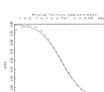
where the parameters values area"0.06, b"0.3,p"0.01 and the initial rate
r0"0.06.
6.1. Call option on zero-coupon bond example
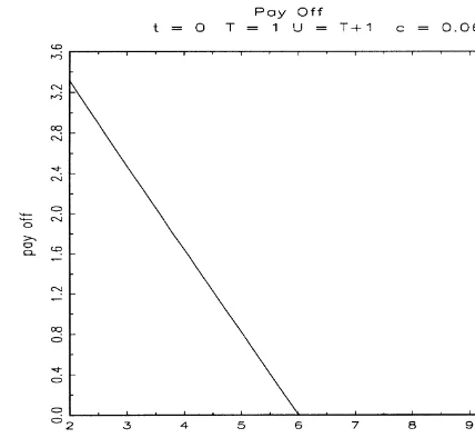
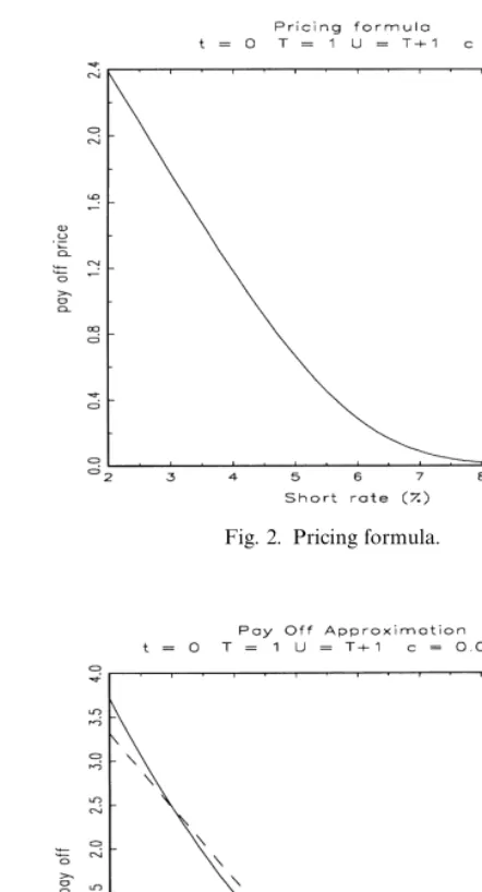
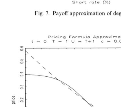
Fig. 1. Payo!pro"le.
8We will further only subscriptrwhen it is necessary to prevent confusion.
prices of European call options on the ;-maturity zero-coupon bond with
exercise rater
k and expiration date ¹4;. We represent in Figs. 1 and 2 the payo!of a call option of maturity¹"1 and strike rater
K"0.06 on a (¹# 1)-maturity zero-coupon bond, and its pricing formula at timet"0.
The computation of the approximated price consists"rst of projecting the payo!onto the basis formed by the Hermite polynomials of order N, ortho-gonal under the marginal law of the factor8 r
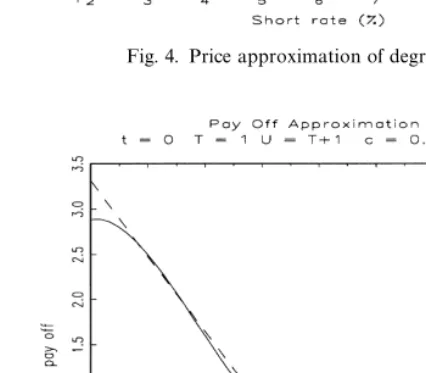
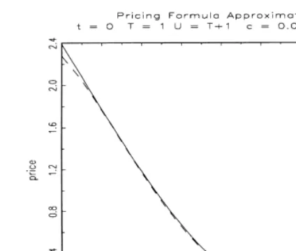
t. Then the approximated price corresponds to the price of the approximated payo!. Figs. 3}6 give two exam-ples of this method, for two choices of the dimension of the space on which we project the payo!. We represent the approximated and the true payo!s, and the corresponding pricing formulas.
At this point, we see that, for a call with a long maturity (one year in our example), the price approximation of degree 2 (delta/gamma approximation) has some good properties (see Fig. 3). Due to the smoothing e!ect of the pricing operator, this ensures a good approximation to the pricing formula (see Fig. 4). As an example, Figs. 5 and 6 show the payo!and the pricing formula approxi-mations when using polynomials of higher order. We see that, for a call payo!, the increase in accuracy is rather small and that a second degree approximation may seem reasonable.
These"gures allow us to make the following six comments:
1. The accuracy of the price approximation decreases when the interest rate
Fig. 2. Pricing formula.
Fig. 3. Payo!approximation of degree 2.
function centered on the mean ofr(i.e. the marginal density ofr) to compute the best approximation.
Fig. 4. Price approximation of degree 2.
Fig. 5. Payo!approximation of degree 5.
pricing formulas because of the regularization properties of the pricing operator.
Fig. 6. Price approximation of degree 5.
4. The smoothing e!ect may be analyzed as follows. Since
DD<P!<P"P
EDD2" = + i/N`1
j2P i ,
and 04j
i41, we see that we get better approximations of the pricing operator corresponding to payo!s being paid far-away (DD<P!<P"P
EDD de-creases inP).
5. From the proof of Theorem 4.1, we can state that
sup f|L2
D<(f)!<"P
E(f)D2
DfD2 4DD<!<"PEDD2.
Thus, it is possible to give an upper bound on the error of the pricing formula that is independent on the payo!.
6. Now, let us compare, for a given payo!, the errors of the pricing formula D<(f)!<"P
E(f)D and of the payo! D(I!PE)(f)D. We can write
f"+=
i/1Sf,eiTei, whereei are the eigenfunctions of<. Then
D<(f)!<"P
E(f)D2" = + i/N`1
j2
iSf,eiT24j2N`1D(I!PE)(f)D2,
since the sequencej
i, i"1,2, is decreasing. We know that in the case of Vasicek modelj
i"exp(!bi). Thus, D<(f)!<"P
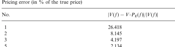
Table 1
Pricing error (in % of the true price)
No. D<(f)!<"P
E(f)D/D<(f)D
1 26.418
2 8.145
3 4.197
5 2.134
7 1.595
10 0.634
We have then obtained a uniform upper bound for the pricing error in our Vasicek example. There is a sharp decline in the approximation error of the pricing formula.
It is clear that the pricing error decreases when the dimension of the approxi-mation space increases. To have a more exact idea of the validity of the projection approach, we compute the pricing error normD<(f)!<"P
E(f)Dfor di!erent choices of the dimension ofE, wherefis the payo!of the call option on a zero-coupon bond. We obtain results given in Table 1.
6.2. Call spread example
Let us now consider a call spread option built from the previous example by buying a European call option with strike rater
k"0.06 and by selling a Euro-pean call option with strike rater
k"0.055.
As in the previous subsection, the two call options are on the ;-maturity
zero-coupon bond and have an expiration date¹4;. We "x the maturities
¹"1 and;"¹#1. The true price is computed as the di!erence of the two call option prices given by the closed-form formula available for European call options on zero coupon bonds.
Figs. 7 and 8 represent the approximated and the true payo!s, and the corresponding pricing formulas. In this example the price approximation of order two does not have good properties, due to the high nonlinearity of the payo!. We need to use a higher order approximation to obtain better results (see Figs. 9 and 10).
Fig. 7. Payo!approximation of degree 2.
Fig. 8. Price approximation of degree 2.
7. Conclusion
Fig. 9. Payo!approximation of degree 5.
Fig. 10. Price approximation of degree 5.
portfolios: our approximation ensures that value at risk is well approximated. It is easy to aggregate a new product in a portfolio by simply adding its approxi-mation. We are able to deal with options of several maturities. At least we can provide upper bounds on the approximation error due to the uniform conver-gence property. Extensions to other cases such as the Cox, Ingersoll and Ross model or multifactor models may also be considered within our framework.
Appendix A. Proofs
A.1. Proof of Theorem 4.1
We consider an Hilbertian basis w
i, i"1,2, of the space ¸2. This basis allows us to build an orthogonal basis w
ij, i,j"1,2, of L2 by setting
w
ij"wi?wj. LetEbe theN-dimensional subspace of¸2generated by the"rst
Nelements of the basisw
i,i"1,2,N, andPEthe projection operator on this subspace. For any linear bounded operator<, with kernelk, satisfying
Assump-tions 3.2 and 3.3,<"P
E is also an integral operator, and we have DD<!<"P
EDD2"Dk!kED2, wherek
Eis theN-rank kernel associated with<"PE. From the decomposition
(3.1) and (4.1) of kernelskandk
Using property (3.2), we have the convergence to zero of the series += ation of the supremum norm:
sup f|L2
D<(f)!<"P
E(f)D2
DfD2 4DD<!<"PEDD2,
A.2. Proof of Lemma 4.1
We consider an Hilbertian basis w
i, i"1,2, of the space ¸2. This basis allows us to build an orthogonal basis w
ij, i,j"1,2, of L2 by setting
w
ij"wi?wj. LetEbe theN-dimensional subspace of¸2generated by the"rst
Nelements of the basisw
i,i"1,2,N, andPEthe projection operator on this subspace. So, for any linear bounded operator <, with kernel k, satisfying
Assumptions 3.2 and 3.3, we have
DD<"P of Theorem 4.1, we have
DD<!<"P
The summation of the two previous terms gives us the equality
DD<DD2"DD<"P
EDD2#DD<!<"PEDD2.
A.3. Proof of Theorem 4.2
We consider an Hilbertian basisw
i,i"1,2, of the space¸2. Looking for the subspace E, the solution of problem (4.2) is equivalent to looking for the subspace solution to the problem (4.3), using Corollary 4.1. We writeI"DD<DD2
andI(E)"DD<"P
EDD2. Properties of the norm give us directlyI"I(E)#I(EM). Rewriting the criterionI(E) in terms of operator<gives us
I(E)"+N
and the problem to solve is then
Max
We are going to build iteratively theN-dimensional optimal projection space. Suppose anN!1-dimensional optimal projection space is built with the"rst
N!1 eigenfunctions of the operator<H<, then
LetEbe anyN-dimensional subspace of¸2. ThenI(E) can be decomposed:
wherepis the dimension of the spaceP
E(EN~1), and
because the sequence of eigenvalues is strictly decreasing, we have
I(E)4+N i/1
j2 i,
for anyN-dimensional spaceE. The supremum is reached if we choose the space of the "rst N eigenfunctions, which is the N-dimensional projection space maximizingI(E).
A.4. Proof of Corollary 4.2
Consider<, an operator, satisfying Assumptions 3.2 and 3.3, and the subspace Eof¸2generated by the"rstNelementsw
i,i"1,2,N, of an Hilbertian basis, then, following the proof of Theorem 4.2, we have to maximize the criterion
IM(E)"DDP tions of<H<associated with the eigenvalueso
i, theno~1@2i <wi,i"1,2,N, are the"rstNeigenfunctions of <<Hassociated with the same eigenvalues, These
A.5. Proof of Corollary 4.3
Consider<, a self-adjoint operator, satisfying Assumptions 3.2 and 3.3, and
the subspaceEof¸2generated by the"rstNeigenfunctionsw
i,i"1,2,N, of
<, then, following Theorem 4.2 and Corollary 4.2, we have directly, for anyf
in¸2
because operators<and<H<have the same eigenfunctions in the self-adjoint
case. Noting that the eigenfunctionw
i has eigenvalueji, we can write
A.6. Proof of Corollary 4.4
Consider<, an operator, satisfying Assumptions 3.2 and 3.3, and the subspace Eof¸2generated by the"rstNelementsw
i,i"1,2,N, of an Hilbertian basis.
P
E"<"PE is the integral operator with kernel:
kx
Following the proof of Theorem 4.2, we have to maximize the criterion
Ix(E)"DDP
The solution of this problem is the space generated by theN"rst eigenfunc-tions of<H<(see Riesz and Nagy, 1990, Chapter 6, p. 243).
References
Abken, P., Madan, D., Ramamurtie, S., 1996. Estimation of risk-neutral and statistical densities by Hermite polynomial approximation: with an application to Eurodollar futures options. Working Paper 96-5, F.E.D. of Atlanta.
Amershi, A.H., 1985. A complete analysis of full Pareto e$ciency in"nancial markets for arbitrary preferences. Journal of Finance 40, 1235}1243.
Bansal, R., Viswanathan, S., 1993a. No arbitrage and arbitrage pricing: a new approach. Journal of Finance 48, 1231}1262.
Bansal, R., Hsieh, D., Viswanathan, S., 1993b. A new approach to international arbitrage pricing. Journal of Finance 48, 1719}1747.
Darolles, S., Florens, J.P., Renault, E., 1998. Nonlinear principal components and inference on a conditional expectation operator. Discussion Paper, CREST.
Darolles, S., GourieHroux, C., 1997. Truncated dynamics and estimation of di!usion equations. Discussion Paper 9736, CREST.
Davies, E.B., 1980. One-Parameter Semi-Groups. Academic Press, New York.
Dunford, N., Schwartz, J.T., 1988. Linear Operators, Part I: General Theory. Wiley, New York. Florens, J.P., Renault, E., Touzi, N., 1998. Testing for embeddability by stationary reversible
continuous-time Markov processes. Econometric Theory 14, 744}769.
Hansen, L., Jagannathan, R., 1997. Assessing speci"cation errors in stochastic discount factor models. Journal of Finance 52, 557}590.
Hansen, L., Scheinkman, J., 1995. Back to the future: generating moment implications for continu-ous time Markov processes. Econometrica 63, 767}807.
Hansen, L., Scheinkman, J., Touzi, N., 1998. Spectral methods for identifying scalar di!usions. Journal of Econometrics 86, 1}32.
Holland, S., 1990. Applied Analysis by the Hilbert Space Method. Marcel Dekker, New York. Jamshidian, F., 1989. An exact bond option formula. The Journal of Finance 44, 205}209. John, K., 1981. E$cient funds in a"nancial market with options: a new irrelevant proposition.
Journal of Finance 36, 685}695.
John, K., 1984. Market resolution and valuation in incomplete markets. Journal of Financial Economics 13, 91}113.
Lacoste, V., 1996. Wiener chaos: a new approach to option hedging. Mathematical Finance 6, 197}213.
Madan, D., Milne, F., 1994. Contingent claims valued and hedged by pricing and investing in a basis. Mathematical Finance 3, 223}245.
Riesz, F., Nagy, B., 1990. Functional Analysis. Dover, New York.
Vasicek, O., 1977. An equilibrium characterization of the term structure. Journal of Financial Economics 5, 177}188.