24 (2000) 1783}1827
The valuation of American barrier options
using the decomposition technique
qBin Gao
!,
*
, Jing-zhi Huang
"
, Marti Subrahmanyam
#
!Kenan-Flagler Business School, University of North Carolina, Chapel Hill, NC 27599, USA"Smeal College of Business, Penn State University, University Park, PA 16802, USA
#Stern School of Business, New York University, New York, NY 10012, USA
Abstract
In this paper, we propose an alternative approach for pricing and hedging American barrier options. Speci"cally, we obtain an analytic representation for the value and hedge parameters of barrier options, using the decomposition technique of separating the European option value from the early exercise premium. This allows us to identify some new put-call&symmetry'relations and the homogeneity in price parameters of the optimal exercise boundary. These properties can be utilized to increase the computational e$ciency of our method in pricing and hedging American options. Our implementation of the obtained solution indicates that the proposed approach is both e$cient and accurate in computing option values and option hedge parameters. Our numerical results also demonstrate that the approach dominates the existing lattice methods in both accuracy and e$ciency. In particular, the method is free of the di$culty that existing
q
This is a substantially revised version of an earlier paper circulated under the title&Analytical Approach to the Valuation of American Path-Dependent Options'. We acknowledge comments and suggestions from two anonymous referees that were extremely useful in revising earlier drafts of this paper. We also acknowledge the extensive and detailed comments of the editor, Michael Selby, that helped to improve the paper substantially, in terms of both content and exposition. We thank James Bodurtha, Jr., Young-Ho Eom, Nengjiu Ju, A.R. Radhakrishnan, Rangarajan Sundaram, and especially Sanjiv Das for comments and discussions, and participants at the Courant Institute Mathematical Finance Seminar (March 1996), the First Annual Computational Finance Conference at Stanford University (August 1996), and the Cornell-Queen's Conference on Derivatives (May 1997) for comments on earlier drafts of the paper.
*Corresponding author. Tel.: (919) 962-7182; fax: (919) 962-2068.
E-mail addresses: [email protected] (B. Gao), [email protected] (J.-Z. Huang), [email protected] (M. Subrahmanyam).
1A recent estimate cited by Hsu (1997) computes the size of the barrier options market to be over 2 trillion dollars in 1996. The market has grown considerably since that time.
numerical methods have in dealing with spot prices in the proximity of the barrier, the case where the barrier options are most problematic. ( 2000 Elsevier Science B.V. All rights reserved.
Keywords: Asset pricing; Derivatives; American option
1. Introduction
Non-standard or exotic options are widely used today by banks, corporations and institutional investors, in their management of risk. The main reason for their popularity is that although standard put and call options are useful risk manage-ment tools, they may not be suitable for hedging certain types of risks. For instance, a corporation may wish to control its raw material costs by limiting the average price paid for a commodity over time (Asian options), or obtaining protection, contingent upon the price breaching a barrier (barrier options). In these and other situations, the use of standard options may involve over-hedging (i.e. providing protection against risks that need not be hedged), and hence higher costs. Consequently, the use of non-standard options may not only"t the risk to be hedged better, but also lower the hedging cost, in such cases.
Although the payo! functions of non-standard options are often not more complex than that of standard options, this is not true for the pricing and hedging of such options. In most cases, such as Asian, barrier and look-back options, whose payo!s are path-dependent, closed-form solutions are hard to come by. This is true even for European-style contracts, except for the special case where the underlying asset price follows a geometric Brownian motion. Therefore, numerical schemes have to be used to calculate the option prices and hedge parameters for American-style options and even for some European-style options.
2In a recent paper, Rogers and Stapleton (1998) provide an alternative lattice-based method for the valuation of barrier options, in which the number of time steps taken is random. However, they implement their method only for the case of European barrier options and standard American options.
speculators, who have a directional view, to obtain a somewhat less expensive directional play on an underlying asset. In some instances, barrier options are American style. Barrier options also include&capped'options as special cases.
Common approaches to option valuation and hedging such as lattice and simulation methods can be problematic when applied to barrier options. It is known that for such options, the binomial method is subject to severe conver-gence problems, and consequently, can lead to huge errors even with a large number of time-steps. The reason is that the payo!of a barrier option is very sensitive to the position of the barrier in the lattice * a &knockout' option behaves very much like a standard option when the underlying asset price is far away from the barrier, but has a near-zero&expected'payo!, when it is close to the barrier.
Boyle and Lau (1994) and Ritchken (1995) develop a restricted bi-nomial/trinomial method to overcome the problem. However, with these methods, it is still extremely di$cult to achieve convergence when the barrier is close to the current price of the underlying asset (the&near-barrier'problem). Gao (1996) proposes an&adaptive mesh'method, which overcomes some of the problems posed by the above models. Even with this modi"cation, the computa-tional time increases as the current underlying price gets closer to the barrier, although at a much slower pace. Further, as shown by Gao, the computational intensity of lattice methods is proportional to the maturity and the square of the volatility. Consequently, the computational costs associated with pricing long maturity and high volatility contracts can be prohibitively high. Cheuk and Vorst (1996) show that a trinomial lattice with a#exible drift can alleviate the
&near-barrier' problem. However, the method permits probabilities to become negative, and can produce fairly large pricing errors for long-term contracts when volatility is high and the spot price is close to the barrier.2
3Hansen and Jorgensen (1997) apply the method to#oating-strike Asian options.
barrier prices, translational invariance in time, and monotonicity in time, and monotonicity in the strike and barrier prices. As mentioned later on, these properties are important in the practical implementation of the method we propose, since the boundary does not have to be recomputed separately for each option.
Our method of implementing the analytic representation using the decompo-sition technique allows us to calculate both option prices and hedge parameters e$ciently and accurately. For example, in the case of American &up-and-out'
options, our numerical results indicate that the approach outperforms both the Ritchken (1995) method and the Cheuk and Vorst (1996) model. In particular, the method we propose is faster than the Ritchken method by two orders of magnitude for equally accurate prices and hedge ratios, when the underlying asset price is close to the barrier. Moreover, in contrast with the other methods, the computational time required by the analytic approach hardly increases as the current underlying asset price gets closer to the barrier. In fact, this& near-barrier'problem, which is endemic in the lattice methods, is completely elimi-nated in our formulation. This is because the optimal exercise boundary, the su$cient input function of our valuation formula, isindependentof the current underlying price. The method proposed here also applies to &capped' options and might be extended to other types of path-dependent options, such as Asian options, whose payo!functions have a Markovian representation in the state space of low dimensionality.3
The paper is organized as follows. In Section 2, an analytic representation is derived"rst for the option price and hedge parameters under the assumption that the underlying asset price process follows a geometric Brownian motion. Put-call &symmetry' conditions and some properties of the optimal exercise boundary are then identi"ed that extend the analytic results to a whole range of related barrier options. Section 3 discusses the implementation of the quasi-analytic formulae and presents our numerical results. Section 4 concludes the paper.
2. A pricing model
In this section, we "rst obtain an analytic representation for the price of American barrier options using the decomposition technique. Based on this representation, we then derive some properties of the optimal exercise boundary.
4See also Geske and Johnson (1984), Selby and Hodges (1987), and Schroder (1989).
American option into that of a similar European option and the early exercise premium. This approach was further developed and speci"c results were ob-tained for the case of the log-normal underlying price process by Kim (1990), Jacka (1991), Carr et al. (1992), and Ho et al. (1997a). Speci"cally, an American option can be considered as a sum of two sets of cash#ows using the decomposi-tion approach: the value of the terminal cash#ow at expiration and the value of the intermediate cash#ows between the valuation date and expiration date.4
The former represents the value of an otherwise identical European option, and the latter, the value of the exercise privilege associated with an American option. Under the risk-neutral pricing framework, the value of an American option is equal to the sum of the expectation of these cash #ows discounted by the risk-free rate.
Before proceeding with the analysis, we "rst de"ne our notation as follows:
c price of a standard European call option C price of a standard American call option c
j price of a non-standard European call option of typean je.g.,&j"uo'denotes
&up-and-out'barrier option C
j price of a non-standard American call option of typej p price of a standard European put option
P price of a standard American put option p
j price of a non-standard European put option of typej P
j price of a non-standard American put option of typej
We also use a superscript&o'to denote standard options. For instance,C0and c0represents the price of a standard American option and a standard European call option, respectively. A superscript&p'denotes the American premium due to the early exercise feature. We also make some assumptions that are common in the option pricing literature as follows:
Assumption 1. The capital market is complete and perfect. Trading takes place continuously and without transaction costs.
5The analysis can be extended to the case of a time-varying (deterministic) interest rate and dividend yield. In principle, the e!ect of stochastic interest rates can also be incorporated into the analysis along the lines proposed by Ho et al. (1997a), although the details of the implementation are likely to be complex.
6The available empirical evidence suggests that this assumption may not always be a good one. Nonetheless, the log-normal case can serve as a benchmark, since the Black and Scholes (1973) model, which is based on this assumption, is widely used and understood in practice. The analysis presented here can be extended to the case of time-varying (deterministic) volatility. However, the case of stochastic volatility would involve additional complexities, as in the case of standard options. Assumption 2. There are two tradeable assets in the market, a risky asset and a riskless asset. The continuously compounded interest rateris constant.5The risky asset pays a constant dividend yield of d50, and its price process
MS
t; t50Nfollows a geometric Brownian motion.6Namely, dS
t"St(r!d) dt#pStd=t (1)
wheredandpare constants, and= is a one-dimensional standard Brownian
motion.
As shown later on, one advantage of making this assumption is that we can obtain an explicit expression for the early exercise premium, and as a result, a quasi-analytic solution for the price of an American barrier option, for instance, an&up-and-out'put option. Consequently, we can perform compara-tive statics analysis and examine analytically the properties of the optimal exercise boundary. We can also derive a put-call &symmetry' relation which allows us to extend the pricing models to a whole set of barrier options.
Without loss of generality, we consider an American-style&up-and-out' put option on the risky asset with a strike priceK, a barrierH, maturity ¹, and a payo! h(S
t)"(K!St)`. The non-standard feature here is that if the asset price &hits' a barrier, the option becomes worthless. (Unless otherwise stated, a zero rebate is assumed throughout the paper, for simplicity. It is relatively easy to relax this assumption.)
Two cases are worth analyzing here: (a)H'K (out-of-the-money& up-and-out'); (b) H4K (in-the-money (at-the-money)&up-and-out'). Note that in the terminology of barrier options &in-the-money' or &out-of-the-money' are not related to the usual de"nition whereS(KorS'K.
2.1. Out-of-the-money&up-and-out'puts
We consider out-of-the-money American &up-and-out' put options, case (a) above, in this subsection. Assume there exists an option pricing function s.t. G: R
7Merton (1973)"rst pointed this out in the case of the American options, both standard and
As demonstrated in McKean (1965) and van Moerbeke (1976), the American option problem can be converted into a free-boundary problem. Under this formalization,G(S
t,t) is the solution to the following problem [see Du$e (1992,
p. 125) for details on the regularity conditions on functionsGandh]:
(D4!r)G(S
where the operatorD4is de"ned as follows:
D4"L
Theorem 1. Consider an American-style&up-and-out'put option withH'K,whose payowupon exercise ish(S
t)"(K!St)` ∀t3 [0,¹].The price of the option is
Note that the last term on the right-hand side (RHS) of (8) indicates that the incremental gain over the time interval [t,t#dt] from exercising the option attis (rK!dS
t) dt. Similarly, the incremental gain from exercising a call option whose payo!is (S
t!K)`is (dSt!rK) dt. Since this gain becomes negative whend"0,
8This amounts to assuming that the boundary consists only of a single piece. This is expected to hold given that the underlying follows a geometric Brownian motion. Our numerical studies also support the validity of the assumption (cf. Tables 1 and 2 and Fig. 1). However, a rigorous justi"cation of this assumption remains to be provided.
9The case of a non-zero dividend yield is considered in the proof of the general formula in Appendix A.
Eq. (8) provides an analytical representation for the price of an American
&up-and-out'put option. However, in order to facilitate the implementation of the formula, it would be desirable to have an explicit expression for the expectation E[)] in (8). This, in turn, depends on the shape of the optimal
exercise boundary LC. We assume that the boundary can be represented by
a continuous functionB160: [0,¹]PR
``.8
Corollary 1. Suppose the underlying asset pays no dividend.9 The price of an American&up-and-out'put option with the barrier levelH'Kis given by
P
60(S0,K)"p60(S0,K)#
P
T
0
rK e~rtPr(S
t4B160,t;Mt0(H) dt (9)
wherePr())is the risk-neutral probability,Mtt21 is the running maximum as dexned
before,and the argument(S
0,K)is used to emphasize that the option isvalued at time0with the underlying asset price equal toS
0 and a strike priceK. The optimal exercise boundary B160"MB160
,t; t3[0,¹]N is determined by the
following condition:
K!B160,
t" lim StsB160,t
P
60(St,K), Mt0(H, ∀t3[0,¹] (10)
Proof. We have that the exercise eventM(S
t,t)3StN"MSt4B160,tNand dividend
d"0. Substituting these into (8) yields (9). h
We now provide further analytical results for the case of out-of-the-money
&up-and-out' put options, on which the implementation (discussed later on in Section 3) is based.
We de"ne the notation as follows:
k,r!p2/2, j,(r#p2/2)/p2,
d
2(x,y,t),(ln(x/y)#kt)/pJt, d1(x,y,t),d2(x,y,t)#pJt,
2.1.1. Option prices and hedge parameters
As discussed before, the price of an American&up-and-out'put option can be written as follows:
P
60(S0,K)"p60(S0,K)#P160(S0,K) (11)
where p
60 and P160 are the prices of the corresponding European option and the early exercise premium, respectively. Speci"cally, the price of the European&up-and-out'put option can be written as (see Rubinstein and Reiner, 1991):
p
60(S0,K)"p0(S0,K)!p6*(S0,K)
"p0(S
0,K)!(H/S0)2j~2p0(H2/S0,K) (12)
where p0(x,K) denotes the Black}Scholes price of a standard European put option with current underlying price x and strike price K, and p
6*())
represents the price of a European up-and-in put option. Following Black and Cox (1976) (Eq. (7)) (see also Cox and Miller (1965, p. 221, Eq. (71))),
where N()) represents the cumulative standard normal function. Thus the
American premium of an&up-and-out'put option is given by
P160"
P
TNotice that the "rst term on the RHS of (13) is the exercise premium of a standard American put option and, as expected, the second term on the RHS goes to zero asHCR.
The hedge parameters can be calculated in a straightforward fashion from (11). For instance, the delta is
10Derman et al. (1995) and Carr et al. (1998) demonstrate that one can use the property of put-call parity to construct a portfolio consisting of a put and a call to statically hedge European barrier options.
and (for the American premium part)
LP160
In the above, n()) is the standard normal density function. One can show that,
similar to the option price, the delta of an American&up-and-out'option also collapses to that of a standard American option as the barrier goes to in"nity. Formulae for other hedge parameters (e.g. gamma, vega, rho, etc.) can be obtained similarly by di!erentiating (11) accordingly and are not presented here in the interest of brevity.
It has been generally recognized that the hedging of barrier options is more di$cult than that of standard options.10 This is mainly due to the unstable properties of the hedge parameters of barrier options, especially near the barrier. The formulae developed here allow us to analytically examine these properties and provide an approach to computing the hedge parameters that is free of the
&near-barrier'problem.
2.1.2. The optimal exercise boundary
We now examine the properties of the optimal exercise boundary. It follows from (10) that the boundaryMB160,
monotonicity in time. We now demonstrate that the exercise boundary (for both standard and non-standard options) has two additional properties. One is homogeneity of degree one in the strike price and the barrier level and the other is translational invariance in time. As shown later, these two properties, com-bined with the fact that the boundary is independent of the underlying asset price, have important implications for the implementation of a pricing model for American options.
Theorem 2. For American barrier options with a strike levelKand a barrierH,the optimal exercise boundary has the following properties:
(a) (Homogeneity of degree one in strike and barrier prices)
B160
,t(jK,jH)"jB160,t(K,H) ∀j'0,t3[0,¹]. (19)
(b) (Translational invariance)
B160
,t~(T2~T1)(K,H,¹1)"B160,t(K,H,¹2) ∀t3[¹2!¹1,¹2]. (20)
(c) (Monotonicity in time)
LB160
,t/Lt'0, t3[0,¹). (21)
(d) (Monotonicity in the barrier level)
LB160,
t/LH(0, t3[0,¹]. (22)
Proof. See Appendix B. h
From the proofs, one can see that the translational invariance in time should hold for any American option with a stationary process for the underlying asset price. The monotonicity is valid as long as the reward for stopping equals K!S
t. The homogeneity follows from the homogeneity of the option pricing function and relies on the log-normality assumption on the underlying process and the assumption that the payo!functionh()) is homogeneous of degree one
in (K,H).
For the sake of completeness, we state the following corollary without proof.
Corollary 2. For standard American(put)options with a strike levelK,the optimal exercise boundary has the following properties:
(a) (Homogeneity in strike)
11To some extent, the implication of the homogeneity of the optimal exercise boundary on the underlying price process can be studied by examining the possible restrictions on the underlying process imposed by the homogeneity of the option pricing function. This is because the former homogeneity comes from the latter homogeneity. Furthermore, to study the necessary conditions for homogeneity, it is enough to consider the case of European options.
As shown in Merton (1973), for a standard European option, a return distribution that is independent of the initial price level is, in general, su$cient for the option price to be homogeneous of degree one in (S,K). [Merton (1990, pp. 306}307) provides a counterexample for this su$ciency condition.] We conjecture that this condition on the return distribution may also be necessary for the homogeneity of the option price in a one-factor continuous-time setting.
12See also Schroder (1997).
(b) (Translational invariance)
B1t~(T2~T1)(K,¹
1)"B1t(K,¹2) ∀t3[¹2!¹1,¹2]. (24)
(c) (Monotonicity in time)
LB1t/Lt'0, t3[0,¹). (25)
Theorem 2 and Corollary 2 show the su$ciency of the log-normality assump-tions for the homogeneity of the optimal exercise boundary (and the homogen-eity of the option pricing function). Whereas the su$ciency has been discussed in the literature (see below), to the best of our knowledge, necessity has not been established. Indeed, the homogeneity of the pricing function is sometimes
assumedto hold in order to simplify the problem.11
2.1.3. Put-call&symmetry'
Chesney and Gibson (1993) and McDonald and Schroder (1998) show that a put-call &symmetry' condition holds for standard American options.12
Namely,
C(S
t,K,d,r)"P(K,St,r,d), (26)
B#t(K,r,d)"K2/B1t(K,d,r), (27)
where B#t()) and B1t()) denote the optimal exercise boundary point at time
t of a standard American call and put option, respectively. Notice that, givenK,d,r,pandt, bothB#t()) andB1
t()) are independent of the spot priceSt. In other words, the exercise decision is made independently of the current spot price. We now demonstrate that a similar relation holds for American barrier options.
following relationships hold:
C
$0(S0,K,H,r,d)"P60(K,S0,KS0/H,d,r), (28)
B#$0
,t(K,H,r,d)"K2/B160,t(K,K2/H,d,r) (29)
where the superscriptscandpdenote call and put,respectively.
Proof. See Appendix C. h
The intuition behind this&symmetry'relation is as follows. We know that the put-call &symmetry' holds for standard options. For &knock-out' options, the additional feature is the&knock-out' provision. Hence, the di!erence between the value of a&knock-out'option and the value of the corresponding standard option depends only on the likelihood of the asset price breaching the barrier. The likelihood of breaching the barrier is determined by the distance between the stock price and the barrier, and the drift of stock price. Under the assump-tion that the stock price follows a log-normal di!usion, the asset price of the
&down-and-out'call drifts away from the barrier at the speed ofr!d. For the put option, the drift isd!r. Since the barrier is above the stock price in this case, the stock price again drifts towards the barrier at the speed ofd!r, in another words, away from the barrier at the speed ofr!d, the same speed as in the call option case. Given that the drifts in the two cases are the same, we also require that the distances between the logarithm of the stock price and the logarithm of the barrier be the same. For the call option, the distance is
lnS!lnH, and for the put option, the distance is lnH1!lnK, whereH1is the
equivalent barrier for the put option. Equating the two yields H1"SK/H. Similar equivalent arguments also apply to the optimal exercise condition.
Note that, in principle, log-normality is a su$cient, but not a necessary condition for put-call&symmetry'to hold. However, the&symmetry'requires that a strong restriction be placed on the underlying distribution even in the zero-drift case. In fact, as shown in Carr et al. (1998), the di!usion term has to have a&symmetry' around the current asset price for the argument to go through.
2.2. In-the-money&up-and-out'puts
In this subsection, we consider in-the-money (at-the-money) American& up-and-out'put options. Consider"rst the case of zero dividend yield. Here, we have:
13See case (a) of Appendix D.
14See, for example, Boyle and Turnbull (1989) and Broadie and Detemple (1995) on&capped'call options.
Proof. See Appendix D. h
As in the case of any put option, early exercise allows the holder of the option to capture the time value of money on the early receipt of the exercise price, by giving up the insurance value of the option and the present value of the dividend stream on the underlying asset. As long as there is no insurance value or stream of dividends, this type of put option should be exercised if it is in the money. This is exactly what happens in this case.
It is worth mentioning that Theorem 4 does not carry over to the case of out-of-the-money&knock-out' options. This is because when H'K, an exer-cised position may not have enough cash to cover the short position in the stock when the barrier is breached.13 This observation also shows that the option will be exercised unconditionally, if the rebate amount,R, is less thanK!H,
whenK'H.
Now supposed'0. In this case, it may not be always optimal to exercise an in-the-money &up-and-out' put since the incremental gain over some time-interval dt from exercising the option may be negative. However, we expect Theorem 4 to also hold in the case of&low'dividend yield because of continuity and, in particular, in the case ofd;r.
2.3. Other types of barrier options
So far, in this section, we have examined &up-and-out' put options and
&down-and-out' call options. We now brie#y analyze &up-and-out' call and
&down-and-out'put options. As shown below, these options include &capped'
options as special cases.14
Consider the case of American &up-and-out' call options. At-the-money (H"K) and out-of-the-money (H(K) calls are easy to analyze. One can see that the only possible cash#ows from these options come from rebate at the barrier. As a result, the option value is equal to the discounted rebate times the risk-neutral probability of the underlying price hitting the barrier.
The analysis of in-the-money &up-and-out' calls (H'K) is more involved. Suppose the dividend yielddis zero. Like a standard American call option, an American &up-and-out' call on a non-dividend-paying stock should not be exercised early. This can also be seen from the discussion of Theorem 1. As a result, one should exercise an American&up-and-out'call option at timetonly whenS
15Technically, for the knock-out event and the exercise date to be well de"ned, the option contract is de"ned in a way such that when the asset price"rst touches the barrier, the option holder has the option to either exercise or let the option be knocked out.
16We thank a referee for pointing this out. B#60,(B#60
,t)t|*0,T+. We have B#60,t"H ∀t3[0,¹]. The payo! at the barrier equals H!K. This exercise strategy is optimal as long as the rebate
R4H!K. However, ifR'H!K, then one should never exercise early. In
either case, however, the option value is equal to the value of a European barrier option with an e!ective rebateR@"max(R,H!K).
Now suppose d'0. In this case, the option payo! upon exercise equals (min(S,H)!K)`"min[(S!K)`,H!K]. This payo!is the same as that of an American &capped' call with a constant capH. Let B#,(B#t)
t|*0,T+ be the
exercise boundary of an otherwise identical standard American call option. We have
Theorem 5. Consider an American &up-and-out' call option withH'K.15 If the rebate at the barrier is no more thanH!K,then such a call option is equivalent to an American&capped'call option with a cap equal toH.Furthermore,the exercise boundary of the&up-and-out'call option is
B#60,
t"min(H,B#t) ∀t3[0,¹] (30)
and the optionvalue is given by
C
60(t)"c60(t)#Et
CP
qHt
e~r(u~t)(dS
u!rK)IMSuzB#60,uNdu
D
, t3[0,qH] (31)where c
60(t) denotes the value of the corresponding European &up-and-out' call option with rebateH!K,and the&hitting time'q
H is dexned as follows:
q
H"infMt3[0,¹]DSt5HN
q
H"¹if the event does not occur by¹.
Proof. Given that rebateR4H!K, it is always better to exercise an&
up-and-out' call than to wait for a knock-out. This strategy guarantees a payo! of
H!KatH. It is then obvious that&up-and-out'call and&capped'call options
are equivalent. Eq. (30) follows from Theorem 1 in Broadie and Detemple (1995). The representation in (31) can be obtained via a reparametrization of the pricing formula (4.4) in Broadie and Detemple (1997) for American&capped'exchange options with proportional cap.16 h
Notice that both (30) and (31) apply also to the case of zero dividend. The explicit formula for the European pricec
17See Kim (1990) and Jacka (1991) for details.
Reiner (1991). Sinceq
His, in general, random, the expectation in (31) might not be always carried out explicitly.
The intuition behind Theorem 5 can be conveyed by considering three cases for the location of the barrier levelHrelative to the level of the boundaryB#.
Case(a):H'B#t ∀t3[0,¹]. First, note that whenHCR, an&up-and-out'call
ption is equivalent to an otherwise identical standard American call option, since the probability of being knocked-out goes to zero. As a result, the two options have the same exercise boundary and hence the same value, i.e., lim
Ht=B#60"B#and limHt=C60(S,K,H)"C(S,K), whereB#,(B#t)t|*0,T+
de-notes the exercise boundary of a standard American call option.
Case(b):H3[B#
T,B#0]. Note thatB#t is a decreasing function oft, due to the declining insurance value and time value of money of the exercise price, reaching a minimum at the expiration date ¹, where B#T"max(rK/d,K).17 Assuming that the boundary is continuous, it intersects the barrier levelHat a unique time tH3[0,¹], s.t. B#tH"H. It follows that an &up-and-out' call alive at time
t3[tH,¹] is equivalent to a standard American call option by the argument for Case (a) above. This implies that B#60
,t"B#t ∀t3[tH,¹]. In particular, B#60
,tH"H. SinceB#60,
tis a decreasing function oft,B#60,t5H ∀t3[0,tH]. How-ever, unless exercised, an &up-and-out' call will be knocked out at H. This indicates that B#60 barrier everywhere sinceB#t declines withtand reaches a minimum at¹.
SinceB#60
,tis a decreasing function oft,B#60,t"H ∀t3[0,¹]. In this case, an American&up-and-out'call behaves like a European&up-and-out'call, but with a rebateR"H!K. Thus, the case is similar to the case whered"0.
American&down-and-out' put options can be analyzed in a similar fashion. Consider "rst out-of-the-money (H'K) and at-the-money (H"K) put op-tions. Like out-of-the-money and at-the-money &up-and-out' calls, cash#ows from these options come only from rebate at the barrier. The valuation problem, is therefore, straightforward. Next, consider in-the-money (H(K)& down-and-out' put options. As expected, these options with a rebate R4K!H are equivalent to American&capped'puts with a cap equal toH. LetB1,(B1
t)t|*0,T+
and B1$0,(B1$0
,t)t|*0,T+ denote respectively the exercise boundary of standard
American put and American&down-and-out'put options. We can now state and prove:
then the option can be considered to be an American&capped'put option with a cap equal toH.Furthermore,the optimal exercise boundary of the&down-and-out'put option can be characterized as follows:
B1$0
,t"max(H,B1t) ∀t3[0,¹] (32)
Proof. This theorem follows from arguments similar to those in the above discussion of Theorem 5.
When H(B1
t ∀t3[0,¹], the put will be exercised before the asset price touches the barrier. Hence,B1$0,t"max(H,B1t)"B1t.
When H'B1T"rK/d, where r(d, it is easy to see thatB1$0,T"H. Since B1$0,t is a non-decreasing function in t, B1$0,t"H ∀t3[0,¹]. In this case, the option becomes a European&down-and-out'put with rebateK!H.
WhenH3[B1T,B10], the barrier intersectsB1. Recall thatB1t increases int. It follows that there exists a unique tH
$0"Mt3(0,¹)DB1t"HN. One can see in the time interval [tH
$0,¹] a live American &down-and-out' put option is, in fact, equivalent to a standard American put option. Since B1tH$0"H and B1
$0,t is monotonic int, B1$0,t"H ∀t3[0,tH
$0]. h
The valuation problem in this case can be handled similarly to the case of
&up-and-out'put options in Section 2.1. More speci"cally, a formula similar to (31) can be obtained for pricing American&down-and-out'put options. A sym-metry relation between American &up-and-out' call and &down-and-out' put options similar to (28) and (29) can be also established. Detailed discussions, however, are omitted here for the sake of brevity.
3. Implementation and numerical results
In this section, we focus on American &up-and-out' put options written on non-dividend paying assets and discuss the implementation of the pricing and hedging formulae (11) and (14) given in Section 2.1.1. We then report some numerical results to illustrate the e$ciency and accuracy of our implementation scheme.
3.1. Implementation
The implementation involves two steps. The"rst is to compute the optimal exercise boundaryB. The second is to calculate the option prices or hedge ratios
takingB as input.
18Other recent work on standard American options includes, but not limited to, Breen (1991), Broadie and Detemple (1996), Bunch and Johnson (1992), Carr (1998), Carr and Faguet (1995).
paying assets. One such scheme is to compute the boundary recursively, an idea originally suggested by Kim (1990). Starting withB
T,BT~1is calculated from
(18). Next,B
T~2is calculated, also from (18), takingBTandBT~1as inputs. This
procedure is repeated iteratively until the entire exercise boundary (an approxi-mated one, strictly speaking) is generated. Once the optimal exercise boundary is obtained, the calculation of option prices and hedge ratios is straightforward, involving only a univariate numerical integration. However, this recursive scheme, which is somewhat computation intensive, can be accelerated using analytical approximations of the exercise boundary, at least for the purpose of pricing.
We focus on two approximation schemes developed in the context of stan-dard American options and based on the integral representation of the early exercise premium. One method is to approximate the exercise boundary by a step-function, i.e. to replace the integral in (18) by a simple sum in our case. This is the approach taken in Huang et al. (1996). The other method is to approximate the exercise boundary by an exponential function. This is based on the observation that the exercise boundary of standard American put options has a shape similar to that of an exponential function. Omberg (1987) and Ho et al. (1994, 1997b) use a single-piece exponential function to approximate the exercise boundary. Ju (1998) uses a multi-piece exponential (MPE) function approximation and also utilizes the integral representation of the early exercise premium.18Under both schemes, the approximated boundary can be described by a few parameters. This allows us to directly compute only a few points on the exercise boundary and, as a result, can increase considerably the computational e$ciency. The resulting option prices/hedge ratios can then be used to extrapo-late the true price/hedge ratios to improve the accuracy of the two schemes (cf. Appendix E for more details).
3.1.1. A&Tabulation'approach to pricing options
The implementation procedure described previously also allows for a scheme to increase computational e$ciency in the valuation of multiple contracts written on the same underlying asset.
On a given day, traders typically need to evaluate their options positions several times. This involves computing positions of contracts written on the same underlying asset. These contracts di!er only in their strike price, barrier level and time to expiration. A conventional implementation scheme involves the calculation of the exercise boundary foreachcontract, i.e. for each value of the parameter set (S
t,K,¹!t,p,r,H). However, due to its homogeneity and
19Similar ideas are independently developed in Joubert and Rogers (1997), whose work we were not aware of until several early drafts of our paper were completed.
20Another advantage of computing the exercise boundary"rst is that, given a contract, one can easily determine if it is optimal to exercise right away at the valuation time, sayt
0. Given the exercise
boundary point at t
0, Bt0, one would exercise the option if St04Bt0. In contrast, the use of
alternative methods would require the computation of the option value att
0to make the decision.
See also Brealey et al. (1983) and Selby (1983) for a related discussion.
for only a few values of the parameter set. This avoids some of the problems of repetitive computation of option prices and hedge ratios. As a result, the computational time can be reduced signi"cantly when pricing a basket of options written on the same underlying asset.19 The translational invariance property implies that, among all the contracts considered [characterized by the parameter set (S
t,K,¹!t,p,r,H)], only the boundary for the longest¹!t,
ceteris paribus, needs to be calculated. The homogeneity property suggests that among all the contracts considered, ceteris paribus, for standard American options only the boundary for one value ofK, needs to be calculated, and for American barrier options among the contracts with the same proportional value of (K,H), only the boundary for one set of (K,H) needs to be calculated.20
These observations suggest an approach to the valuation and hedging of American options in which the optimal exercise boundary is tabulated for di!erent values of the parameter set (K,H,¹!t,p,r). Computing the option prices and hedge ratios then amounts to calling a tabulated&exercise boundary'
function.
3.1.2. Optimal exercise boundary
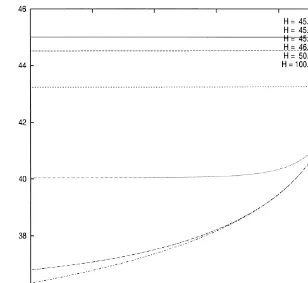
As mentioned earlier, the implementation of the analytic method requires the optimal exercise boundary as an input. In this section, as an illustration, we provide plots of the optimal exercise boundary for American barrier put op-tions. The boundary for American barrier call options can be obtained using the put-call &symmetry' relationship derived earlier. As shown below, useful in-formation can be extracted from such a plot of the optimal exercise boundary. Fig. 1 illustrates the plots of the optimal exercise boundary for American
&up-and-out' put options on non-dividend-paying stocks for di!erent levels of the barrier. Speci"cally, we choose six levels of the barrier, namely, H"45, 45.01, 45.10, 46, 50, 100. The values of the other relevant parameters are
K"45, ¹!t"1,p"0.2, andr"0.0488. One can see that for a givenH, the
Fig. 1. Optimal exercise boundaries of American barrier options with di!erent barrier levels. Fig. 1 shows the plots of the optimal exercise boundary for American out-of-the-money&up-and-out'put options on non-dividend-paying stocks for di!erent values of the barrier level H, namely H"45, 45.01, 45.10, 46, 50, 100. The values of other relevant parameters are: strike priceK"45, time to expiration¹!t"1 (yr), volatilityp"0.2, and risk-free rater"0.0488. The boundary with H"45 coincides with the strike price. The boundary withH"100 is essentially the same as the boundary of an otherwise identical standard American option (H"R). Each boundary shown here is generated using 200 points (time-steps).
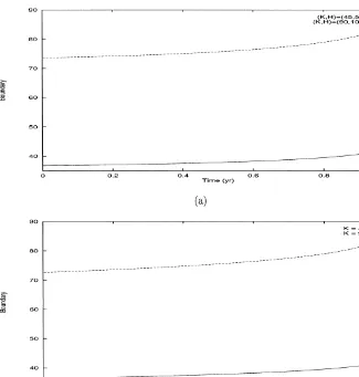
Fig. 2. Price homogeneity of optimal exercise boundaries of American&up-and-out'put options. Fig. 2 illustrates the price homogeneity of the optimal exercise boundary for American out-of-the-money
&up-and-out'put options on non-dividend-paying stocks. Fig. 2(a) shows plots of the boundary with (K"45,H"50) and (K"90,H"100) to illustrate the homogeneity in (K,H). Fig. 2(b) shows plots of the boundary with (K"45,H"100) and (K"90,H"500) to illustrate the homogeneity inKwhenH<Kor essentially whenH"R. In both (a) and (b), the height of the dashed curve is twice the height of the solid curve (homogeneity). The values of other relevant parameters are time to expiration¹!t"1 (yr), volatilityp"0.2, and risk-free rater"0.0488. Each boundary shown here is generated using 200 points (time-steps).
21Gao (1996) discusses the pricing errors from the lattice model. He also shows that non-constant time steps can alleviate the problem only partially.
the homogeneity in (K,H). Fig. 2(b) shows plots of the boundary with (K"45, H"100), the solid curve, and the boundary with (K"90 ,H"500), the dashed curve, to illustrate the homogeneity inK whenH<K. Note that
whenH<K, an&up-and-out'put option is essentially equivalent to a standard
American put option. So Fig. 2(b) actually illustrates the homogeneity inKof optimal exercise boundaries for standard American options. The values of other relevant parameters are time to expiration, ¹!t"1 (yr), volatility, p"0.2, and risk-free rate,r"0.0488. In both (a) and (b), the height of the dashed curve is twice the height of the solid curve, which veri"es the price homogeneity.
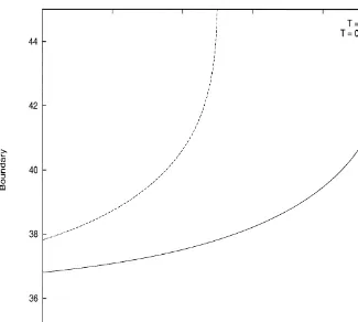
Fig. 3 illustrates the translational invariance of the optimal exercise boundary of American out-of-the-money&up-and-out'put options on non-dividend-pay-ing stocks. Two plots of the boundary are shown in the"gure and di!er only in time to expiration, the dashed curve with¹!t"0.5 (yr) and the solid curve with¹!t"1 (yr). The values of other relevant parameters are strikeK"45, barrierH"50, volatilityp"0.2, and risk-free rater"0.0488. When shifted to the left for ¹!t"0.5, the solid curve will coincide with the dashed curve, which veri"es the stationarity property.
We should emphasize that the method developed here has a de"nite advant-age over the lattice methods in computing the optimal exercise boundary. For instance, it would be very di$cult to obtain a plot as smooth as those shown in Fig. 1 using a lattice method, even with a large number of time steps. In contrast, the plots shown in Fig. 1, for instance, were generated using the analytic formula with 200 points (time-steps) and the amount of the computational time required is about 0.6 s (CPU time) on a Sun Ultra 1 workstation.
3.2. Numerical results
It has been recognized that the simple binomial method is not appropriate for pricing barrier options due to the fact that the price of such options is very sensitive to the location of the barrier in the lattice. The reason for this sensitivity comes from the fact that the option-value function is not smooth around the barrier. The existence of such&kinks'and the discrete price-space in the binomial/trinomial models e!ectively causes a shift of the barrier to a nearby layer of nodes, once the barrier falls in-between two layer of nodes.21
Fig. 3. Stationarity of optimal exercise boundaries of American &up-and-out'put options. Fig. 3 illustrates the stationarity of the optimal exercise boundary of American out-of-the-money
&up-and-out'put options on non-dividend-paying stocks. Two plots of the boundary are shown in the"gure and di!er only in time to expiration, one with ¹!t"0.5 (yr) and the other with ¹!t"1 (yr). When shifted to the right for¹!t"0.5, the dashed curve will coincide with the solid curve (stationarity). The values of other relevant parameters are strikeK"45, barrierH"50, volatilityp"0.2, and risk-free rater"0.0488. Each boundary shown here is generated using 200 points (time-steps).
22Extrapolation methods may be helpful in this case, provided the individual elements in the sequence used for extrapolation (i.e. the option prices) can be computed with reasonable accuracy.
23For instance, consider a contract withS
t"49.9,H"50,K"45,¹!t"5 (yr), andp"0.4, whose true price is&very'close to 0.0634. Our implementation shows that the put value using the Cheuk}Vorst scheme equals 0.09 withN"100, 0.0640 withN"1000, and 0.0634 withN"10,000, respectively. Negative probabilities occur in all three cases.
24In the Ritchken method, the number of time steps cannot be chosen arbitrarily, due to the restriction that the barrier has to coincide with a node [see Ritchken (1995) for details]. In our implementation, the number of time steps used for contract Set I (to be speci"ed below) is between 10,027 and 11,677, and for contract Set II (to be speci"ed below) is between 10,027 and 21,385.
In Cheuk and Vorst, the drift of each trinomial step can vary. When the spot price is close to the barrier, the drift can be adjusted to ensure a reasonably large step-size in the price dimension, which is inversely related to the number of time periods required in the lattice. As a result, the convergence can be improved compared to the Ritchken method. However, for some range of parameter values with a"xed number of time steps, the Cheuk}Vorst scheme can produce negative probabilities and signi"cant pricing errors, especially for long-term contracts with high volatility.23Also, it remains to be shown how to compute hedge ratios using the method when the spot price is near the barrier, because step-sizes in price around the spot price are non-uniform.
The adaptive-mesh method developed by Gao solves the&near-barrier' prob-lem by using a "ner mesh around the barrier while maintaining a coarse structure in other places. It still su!ers from the problem that the number of time steps goes to in"nity as the asset price and the barrier get close to each other, although this happens only near the boundary in the time-price space, as opposed to everywhere in the restricted binomial/trinomial models. In contrast, as shown below, this sensitivity problem can be completely eliminated by using the analytic method developed here.
For a given method, the accuracy is measured by the deviation from a bench-mark, more speci"cally by the root of the mean squared error (RMSE) or the root of the mean squared relative error (RMSRE). The benchmark is chosen to be the results from the Ritchken method with at least ten thousand time steps.24
The e$ciency is measured by the CPU time required to compute option prices or hedge ratios for a given set of contracts. We choose two sets of contracts for comparison. Each set consists of forty-eight contracts that have di!erent values of the underlying asset priceS
tat valuation datet, the time-to-expiration¹!t, and the volatility parameterp. The barrier levelHand the strike valueKare
"xed at 50 and 45, respectively. The risk-free rate r is chosen to be 0.0488. In Set I, we choose S
t"(40, 42.5, 45, 47.5), ¹!t"(0.25, 0.5, 0.75, 1.0), and
p"(0.2, 0.3, 0.4). As a result, the set of contracts include out-of-the-money, at-the-money, and in-the-money options. Set II is similar to Set I, except that those contracts with S
t"47.5 are replaced by contracts with St"49.5. The reason for this choice is to include contracts withS
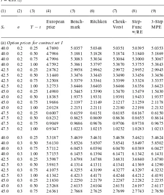
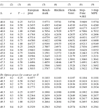
Table 1 summarizes the statistics for option prices for the decomposition method and the trinomial methods in relation to the benchmark (the Ritchken (1995) method with at least ten thousand time-steps). Speci"cally, three schemes for implementing the decomposition method are included (cf. Appendix E for
Table 1
Prices of American&up-and-out'put options on non-dividend-paying stocks (K"$45;H"$50; r"4.88%)!
(1) (2) (3) (4) (5) (6) (7) (8) (9) (10)
European Bench- Ritchken Cheuk} Step-Func
3-Step 3-Step S
t p ¹!t price mark Vorst
w/RE
MPE MPE
w/RE (a)Option prices for contract set I
Table 1 continued
(1) (2) (3) (4) (5) (6) (7) (8) (9) (10)
European Bench- Ritchken Cheuk} Step-Func 40.0 0.4 0.25 5.8723 5.9773 5.9781 5.9796 5.9809 5.9754 5.9778 40.0 0.4 0.50 6.2435 6.4285 6.4244 6.4310 6.4326 6.4260 6.4292 40.0 0.4 0.75 6.3496 6.6162 6.6147 6.6207 6.6173 6.6137 6.6171 40.0 0.4 1.00 6.3540 6.7054 6.7029 6.7077 6.7006 6.7032 6.7063 42.5 0.4 0.25 4.1768 4.2424 4.2438 4.2455 4.2470 4.2406 4.2427 42.5 0.4 0.50 4.5514 4.6759 4.6721 4.6782 4.6831 4.6737 4.6764 42.5 0.4 0.75 4.6580 4.8422 4.8396 4.8451 4.8489 4.8400 4.8427 42.5 0.4 1.00 4.6727 4.9188 4.9155 4.9218 4.9213 4.9169 4.9194 45.0 0.4 0.25 2.6628 2.7007 2.6971 2.7042 2.7036 2.6993 2.7010 45.0 0.4 0.50 2.9602 3.0368 3.0336 3.0383 3.0428 3.0352 3.0370 45.0 0.4 0.75 3.0436 3.1591 3.1572 3.1620 3.1663 3.1576 3.1594 45.0 0.4 1.00 3.0586 3.2145 3.2133 3.2179 3.2195 3.2131 3.2148 47.5 0.4 0.25 1.2875 1.3049 1.3043 1.3081 1.3060 1.3041 1.3050 47.5 0.4 0.50 1.4496 1.4859 1.4846 1.4875 1.4891 1.4851 1.4860 47.5 0.4 0.75 1.4946 1.5500 1.5493 1.5528 1.5543 1.5492 1.5501 47.5 0.4 1.00 1.5035 1.5787 1.5781 1.5822 1.5822 1.5780 1.5788 (b)Option prices for contract set II
49.5 0.2 0.25 0.1077 0.1103 0.1103 0.1107 0.1104 0.1101 0.1103 49.5 0.2 0.50 0.1542 0.1613 0.1613 0.1619 0.1618 0.1611 0.1614 49.5 0.2 0.75 0.1711 0.1828 0.1828 0.1836 0.1839 0.1826 0.1828 49.5 0.2 1.00 0.1773 0.1936 0.1936 0.1945 0.1949 0.1934 0.1936 49.5 0.3 0.25 0.1957 0.1990 0.1990 0.1999 0.1992 0.1988 0.1990 49.5 0.3 0.50 0.2364 0.2439 0.2439 0.2449 0.2446 0.2437 0.2439 49.5 0.3 0.75 0.2489 0.2606 0.2606 0.2619 0.2617 0.2604 0.2606 49.5 0.3 1.00 0.2525 0.2684 0.2684 0.2700 0.2695 0.2682 0.2684 49.5 0.4 0.25 0.2529 0.2563 0.2563 0.2574 0.2565 0.2561 0.2563 49.5 0.4 0.50 0.2859 0.2930 0.2930 0.2944 0.2936 0.2928 0.2930 49.5 0.4 0.75 0.2950 0.3059 0.3059 0.3076 0.3068 0.3057 0.3059 49.5 0.4 1.00 0.2969 0.3117 0.3117 0.3137 0.3124 0.3115 0.3117 !Table 1 reports the values of American&up-and-out'put options on non-dividend-paying stocks for two sets of contracts computed using di!erent methods. Set I includes 48 contracts, each of which has a di!erent value of the parameter set (S
t,¹!t,p). The domain of this parameter set is S
t"(40, 42.5, 45, 47.5),¹!t"(0.25, 0.5, 0.75, 1.0), andp"(0.2, 0.3, 0.4). Set II is similar to set I, except that those contracts withS
t"47.5 are replaced by contracts withSt"49.5. Panels (a) and (b) show the numerical results for contract set I and II, respectively. Columns 1 through 3 represent the values of the parameters,S
25In our implementation of the Ritchken model, the number of time steps used is between 53 and 183 for Set I, and between 55 and 4753 for Set II.
details): (a) using a step-function to approximate the exercise boundary com-bined with a four-point Richardson extrapolation; (b) using a three-piece ex-ponential function to approximate the exercise boundary without extrapolation; and (c) using a three-piece exponential function to approximate the exercise boundary combined with a three-point Richardson extrapolation. For the trinomial methods, the Ritchken (1995) scheme (with a minimum 50 time steps in the trinomial tree)25and the Cheuk}Vorst (1996) method (with the number of time steps N"100) are included for comparison. As can be seen, &penny'
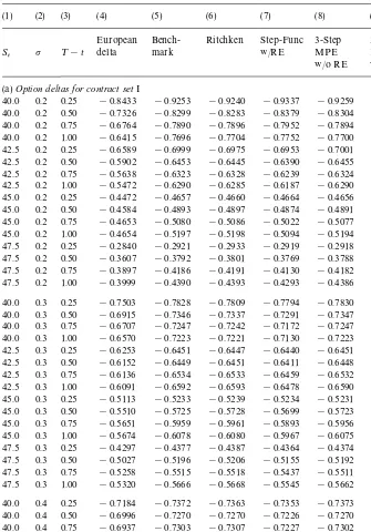
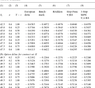
accuracy can be achieved in almost all cases for the values of the option. Table 2 reports the statistics for hedge ratios for the Ritchken method and the three analytical approximations. Like the prices, the hedge ratios are within 0.01 of the benchmark in almost every case. The key issue, therefore is one of computational e$ciency, given a level of accuracy.
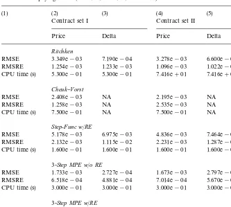
Table 3 summarizes numerical results of the accuracy and speed of computa-tion for opcomputa-tion prices and deltas of our formulae (11) and (14) using the Ritchken method, the Cheuk}Vorst method, and the three approximation schemes men-tioned above for the two sets of contracts. Columns 2 and 3 list the results for the contracts in Set I and columns 4 and 5 for the contracts in Set II. The results for the RMSE and RMSRE for all"ve methods are shown in the table, respectively. The CPU-times, the amount of time required (on a Sun Ultra 1 workstation) to compute the option prices or the delta values for all the forty-eight contracts in each set, are also presented in the table.
One can see from Table 3 that the errors from all the"ve methods are small under either of the two measures* RMSE and RMSRE* for both sets of contracts. The three-step MPE with Richardson extrapolation clearly domin-ates the other methods in terms of accuracy.
Regarding speed, one can see from Table 3 that the step-function approxima-tion is the fastest among the"ve methods. Also, except for the Ritchken method, the CPU-time required for Set II that includes the contracts withS
t"49.5 very close to the barrier (H"50) is basically the same as that for set I. The Ritchken method is strongly dominated by the analytical approximation methods. This indicates that the quasi-analytic method can deal e$ciently with the case in which the underlying price is very close to the barrier. As mentioned earlier, the reason is that the optimal exercise boundary, the su$cient input function of the valuation formula, isindependent of the current underlying price. As a result, the problem of the underlying price being too close to the barrier is completely avoided in our approach.
Table 2
Deltas of American&up-and-out'put options on non-dividend-paying stocks (K"$45;H"$50; r"4.88%)!
(1) (2) (3) (4) (5) (6) (7) (8) (9)
European Bench- Ritchken Step-Func 3-Step MPE
3-Step MPE S
t p ¹!t delta mark w/RE w/o RE w/RE
(a)Option deltas for contract setI
Table 2 continued (b)Option deltas for contract set II
49.5 0.2 0.25 !0.2192 !0.2244 !0.2251 !0.2225 !0.2240 !0.2245 !Table 2 reports the delta values of American&up-and-out'put options on non-dividend-paying stocks for two sets of contracts computed using di!erent methods. Set I includes 48 contracts, each of which has a di!erent value of the parameter set (S
t,¹!t,p). The domain of this parameter set is S
t"(40, 42.5, 45, 47.5),¹!t"(0.25, 0.5, 0.75, 1.0), andp"(0.2, 0.3, 0.4). Set II is similar to set I, except that those contracts withS
t"47.5 are replaced by contracts withSt"49.5. Panels (a) and (b) show the numerical results for contract set I and II, respectively. Columns 1 through 3 represent the values of the parameters,S
t(the time-tstock price),p(volatility), and¹!t(the time to expiration). Column 4 reports the European delta values obtained using the analytic formula in (15). Columns 5 and 6 show the numerical results of delta values from the Ritchken method with at least 10,000 time steps (the benchmark), and the Ritchken method with at least 50 time steps, respectively. Columns 7 through 9 show the numerical results from three analytic approximation techniques: the step-function scheme using a four-point Richardson extrapolation, and the three-step multi-piece exponential (MPE) approximation with and without Richardson extrapolation.
Table 3
Summary of results on option prices and delta values of American&up-and-out'put options on non-dividend-paying stocks (K"$45;H"$50;r"4.88%)!
(1) (2) (3) (4) (5)
Contract set I Contract set II
Price Delta Price Delta
Ritchken
RMSE 3.349e!03 7.190e!04 3.278e!03 6.600e!04 RMSRE 1.254e!03 1.233e!03 1.096e!03 1.022e!03 CPU time (s) 5.300e!01 5.300e!01 7.416e#01 7.416e#01
Cheuk}Vorst
RMSE 2.408e!03 NA 2.195e!03 NA
RMSRE 1.258e!03 NA 2.535e!03 NA
CPU time (s) 7.500e!01 NA 7.500e!01 NA
Step-Func w/RE
RMSE 5.178e!03 6.975e!03 4.836e!03 7.464e!03 RMSRE 2.132e!03 1.115e!02 2.231e!03 1.287e!02 CPU time (s) 1.600e!01 1.600e!01 1.600e!01 1.600e!01
3-Step MPE w/o RE
RMSE 1.733e!03 2.727e!04 1.673e!03 2.797e!04 RMSRE 6.518e!04 4.881e!04 7.014e!04 5.670e!04 CPU time (s) 3.000e!01 3.000e!01 3.000e!01 3.000e!01
3-Step MPE w/RE
RMSE 5.991e!04 1.261e!04 5.937e!04 1.242e!04 RMSRE 1.786e!04 2.047e!04 1.728e!04 2.011e!04 CPU time (s) 5.700e!01 5.700e!01 5.700e!01 5.700e!01
!Table 3 reports a summary of the results from the Ritchken, the Cheuk}Vorst, and the three analytical approximation methods for American&up-and-out'put options on non-dividend-paying stocks for two sets of contracts. Set I includes 48 contracts, each of which has a di!erent value of the parameter set (S
t,¹!t,p). The domain of this parameter set is St"(40, 42.5, 45, 47.5), ¹!t"(0.25, 0.5, 0.75, 1.0), andp"(0.2, 0.3, 0.4). Set II is similar to set I, except that those contracts withS
t"47.5 are replaced by contracts withSt"49.5. Columns 2 and 3 show the numerical results of option prices and delta values for contract set I. Columns 4 and 5 show the numerical results of option prices and delta values for contract set II. Beginning with row 3, deviation from the benchmark*the results from the Ritchken method with at least 10,000 time steps*is reported for each of the following"ve methods: the Ritchken method with at least 50 time steps, the Cheuk and Vorst with 100 time steps, the step-function scheme using a four-point Richardson extrapolation, and the three-step multi-piece exponential (MPE) approximation with and without Richardson extrapolation.
Table 4
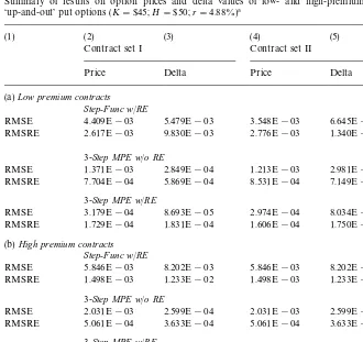
Summary of results on option prices and delta values of low- and high-premium American
&up-and-out'put options (K"$45;H"$50;r"4.88%)!
(1) (2) (3) (4) (5)
Contract set I Contract set II
Price Delta Price Delta
(a)Low premium contracts Step-Func w/RE
RMSE 4.409E!03 5.479E!03 3.548E!03 6.645E!03 RMSRE 2.617E!03 9.830E!03 2.776E!03 1.340E!02
3-Step MPE w/o RE
RMSE 1.371E!03 2.849E!04 1.213E!03 2.981E!04 RMSRE 7.704E!04 5.869E!04 8.531E!04 7.149E!04
3-Step MPE w/RE
RMSE 3.179E!04 8.693E!05 2.974E!04 8.034E!05 RMSRE 1.729E!04 1.831E!04 1.606E!04 1.750E!04 (b)High premium contracts
Step-Func w/RE
RMSE 5.846E!03 8.202E!03 5.846E!03 8.202E!03 RMSRE 1.498E!03 1.233E!02 1.498E!03 1.233E!02
3-Step MPE w/o RE
RMSE 2.031E!03 2.599E!04 2.031E!03 2.599E!04 RMSRE 5.061E!04 3.633E!04 5.061E!04 3.633E!04
3-Step MPE w/RE
RMSE 7.852E!04 1.562E!04 7.852E!04 1.562E!04 RMSRE 1.842E!04 2.241E!04 1.842E!04 2.241E!04
!Table 4 reports a summary of the results from the analytic methods for both low- and high-premium out-of-the-money American &up-and-out'put options on non-dividend-paying stocks for two sets of contracts. Set I includes 48 contracts, each of which has a di!erent value of the parameter set (S
t,¹!t,p). The domain of this parameter set is St"(40, 42.5, 45, 47.5), ¹!t"(0.25, 0.5, 0.75, 1.0), andp"(0.2, 0.3, 0.4). Set II is similar to set I, except that those contracts withS
top half of the group, whereas low-premium contracts within each set are those whose premia ranked in the bottom half. Table 4 reports a summary of the results from the analytic methods between low- and high-premium contracts. Panels (a) and (b) summarize, respectively, the results for low- and high-premium options within each set of contracts. Columns 2 and 3 show the numerical results of option prices and delta values for contract set I. Columns 4 and 5 show the numerical results of option prices and delta values for contract set II. One can see from the table that the step-function scheme basically has lower RMSE but higher RMSRE in low-premium contracts than in high-premium contracts. Roughly, the same pattern holds for the three-step MPE without extrapolation. The three-step MPE extrapolation scheme has both lower RMSE and RMSRE in low-premium contracts than in high-premium contracts. These results seem to indicate that the three-step MPE extrapolation scheme is the most sensitive to the premium among the analytical approxima-tion methods. However, the errors from all three methods are small for both low- and high-premium contracts.
Overall, among the methods considered here, the three-step MPE without Richardson extrapolation seems to provide the best balance between accuracy and computational e$ciency. In summary, our numerical experiments show that the quasi-analytic pricing formula (11) is both accurate and e$cient, and dominates the existing lattice methods. In particular, its performance is robust in the sense that both the accuracy and the e$ciency arenotsensitive to either the American option premium, or to the distance between the underlying price and the barrier.
4. Conclusion
Non-standard or exotic options are in wide-spread use today in global
"nancial markets. Increasingly, over-the-counter options on many assets includ-ing equities,"xed income securities, foreign exchange and commodities have non-standard characteristics, such as the&knock-out'/&knock-in'feature, and the averaging of the price of the underlying asset, among others. Often, due to the lack of liquid secondary markets for such products, in view of their custom-designed nature, an optimal exercise or American-style feature is incorporated into the design of the contract. It is well-known that, even for standard options, the American feature causes problems for valuation and hedging, since there is no closed-form solution for the prices and hedge parameters, in general. There-fore, most models of American option valuation and hedging are implemented using numerical procedures. This problem is further compounded for non-standard American options.
26Recently, Hansen and Jorgensen (1998), applied the decomposition technique to the case of
#oating-strike Asian options.
methods are based on a lattice or grid and the accuracy of the results obtained is limited by the"neness of the grid. For exotic options such as barrier options, whose values are very sensitive to even minor perturbations in the parameters, the errors due to inappropriate lattices may be substantially large, and the computational time necessary to reduce these errors by choosing a"ner grid size may be very intensive. In fast-moving markets, it is obviously essential to obtain reasonably accurate prices and hedge ratios fairly quickly. Another limitation is that even if one can come up with numerical methods that are fairly e$cient and accurate, it is di$cult to obtain an intuitive understanding of how the pricing and hedging works, in the absence of analytical results.
These problems make it desirable, whenever possible, to derive quasi-analyti-cal models for non-standard American options. Our research shows that in many cases, such formulae can be derived, at least for some cases of exotic options, extending the work of Kim (1990), Jacka (1991) and Carr et al. (1992). We are able to derive quasi-analytical formulae for the prices and hedge ratios in the case of barrier options (and&capped'options). The formulae are imple-mented using analytic approximations of the optimal exercise boundary and Richardson extrapolation. Our results indicate that our method is both accurate and e$cient. In particular, the &near-boundary' sensitivity problem associated with using lattice methods is completely eliminated by using the technique developed here.
Our approach also indicates the advantage of studying the optimal exercise boundary when dealing with American options. We identify and exploit two key properties of the optimal exercise boundary*homogeneity in price parameters and translational invariance* for American options. In addition, some new put-call&symmetry'relations are also derived. These properties can be utilized to reduce repetitive computation of option prices and hedge ratios, and hence increase the e$ciency of pricing and hedging American options. We present the details of our approach for American-style barrier options. The approach, based on the decomposition technique, can be applied to other non-standard Ameri-can-style options such as look-back options and Asian options.26
Appendix A. Proof of Theorem 1
Under suitable regularity conditions, we have that the discounted accumulat-ive trading pro"ts from holding an American option from time 0 to timet,
Kt"G(S
t,t)e~rt!G(S0,0)!
P
t
0
Ds[e~ruG(S
is a martingale under the risk-neutral measure [see for example Karatzas and Shreve (1991, p. 328)]. For instance, this holds ifG()) is the pricing function of
standard American options. In the case of barrier options, the option pricing functionG(S
t,t) may not satisfy the usually assumed regularity conditions near
the barrier. However, similar to standard European barrier-option pricing functions,G(S
t,t) should satisfy those regularity conditions in the
non-knock-out region where Mt0(H and which is what we focus on. Based on this argument, we claim that Kt as de"ned above is a martingale when G(S
t,t) represents the price of an&out-of-the-money'American&up-and-out'put option.
It follows that
Substituting (A.3) into (A.2) yields (8) in Theorem 1. This completes the proof. h
Appendix B. Proof of Theorem 2
To simplify the notation, the subscript&uo'inB
60,tis dropped in this appendix and the boundary point attis simply denoted byB
t.
B.1. Homogeneity
We prove this by induction in a discrete-time setting. The assertion is true for B
T given the boundary condition B
T"min[min(rK/d,K),H]. (B.1)
Next considerB
T~1. Neglecting the early exercise premium, we have from (18)
K!B
T~1"p60(BT~1,K,H),
whereHhas been explicitly speci"ed as an argument. One can easily see from this equation that the assertion holds forB
27The uniqueness of the boundary has been assumed implicitly.
wheref()) denotes the integral on the RHS of (18). Under the transformation
hPah ∀a3R
``,
the equation for the transformed boundary pointB
t~1(ah) becomes
aK!B
t~1(ah)"p60(Bt~1(ah),ah)#f(Bt~1(ah),MBu(ah);u5tN,ah) "ap
60(Bt~1(ah)/a,h)#f(Bt~1(ah),MaBu(h);u5tN,ah) "ap
60(Bt~1(ah)/a,h)#af(Bt~1(ah)/a,MBu(h);u5tN,h), (B.2)
where the homogeneity of (B
u)uzthas been used in the second equality. Dividing (B.2) byaon both sides, we have by de"nition27
B
t~1(ah)/a"Bt~1(h),
which says thatB
t~1(h) is homogeneous of degree one inh.
B.2. Translational invariance in time
LetMB
t(K,H,¹);t3[0,¹]Nbe the optimal exercise boundary of a contract
with the expiration date¹. It can be seen from (18) that
B
t(K,H,¹)"Bt~u(K,H,¹!u) ∀04u4t4¹ Given"xed¹
1and¹2 where¹2'¹1, it follows that
B
t(K,H,¹2)"Bt~(T2~T1)(K,H,¹2!(¹2!¹1)) "B
t~(T2~T1)(K,H,¹1) ∀t3[¹2!¹1,¹2].
B.3. Monotonicity in time
Di!erentiating (17) with respect tot on both sides and using the fact that
LP
60/Lt(0 yieldsLBt/Lt'0.
B.4. Monotonicity in the barrier level
Given timet, it is obvious that an option price is an increasing function of the barrier level, i.e.
LP
60(St,H,K)
Given that the optimal boundary condition satis"es
one can take the partial derivative on the two sides, so that
LB
Appendix C. Proof of Theorem 3
We prove the &put-call symmetry' for the case of the out-of-the-money
&knock-out' option only. The case of the in-the-money &knock-out' can be analyzed in a similar fashion.
We de"ne the notation"rst.
d1(x,y,t,r,d)"ln(x/y)#(r!d#p2/2)t
To simplify the notation, we shall omit the subscript&do'or&uo'and useB#t and B1t to denote the optimal exercise boundary of a&down-and-out'call option and an &up-and-out' put option, respectively. Recall also that the superscript &o'