STATISTICAL METHODS IN AI: RARE EVENT LEARNING USING ASSOCIATIVE
RULES AND HIGHER-ORDER STATISTICS
V. Iyer†∗S. Shetty†S.S. Iyengar‡
†Electrical and Computer Engineering, Tennessee State University, Nashville, TN 37210, USA - (viyer, sshetty)@tnstate.edu ‡
School of Computing and Information Sciences, Florida International University, Miami, FL 33199, USA - [email protected]
Commission VI, WG VI/4
KEY WORDS:Hoeffding Bounds, Big Samples, Trajectories, Spatio-Temporal Mining, Statistical Methods, Overlap-Function, AI And Kernel Methods, Random Forest Ensembles
ABSTRACT:
Rare event learning has not been actively researched since lately due to the unavailability of algorithms which deal with big samples. The research addresses spatio-temporal streams from multi-resolution sensors to find actionable items from a perspective of real-time algorithms. This computing framework is independent of the number of input samples, application domain, labelled or label-less streams. A sampling overlap algorithm such as Brooks-Iyengar is used for dealing with noisy sensor streams. We extend the existing noise pre-processing algorithms using Data-Cleaning trees. Pre-processing using ensemble of trees using bagging and multi-target regression showed robustness to random noise and missing data. As spatio-temporal streams are highly statistically correlated, we prove that a temporal window based sampling from sensor data streams converges afternsamples using Hoeffding bounds. Which can be used for fast prediction of new samples in real-time. The Data-cleaning tree model uses a nonparametric node splitting technique, which can be learned in an iterative way which scales linearly in memory consumption for any size input stream. The improved task based ensemble extraction is compared with non-linear computation models using various SVM kernels for speed and accuracy. We show using empirical datasets the explicit rule learning computation is linear in time and is only dependent on the number of leafs present in the tree ensemble. The use of unpruned trees (t) in our proposed ensemble always yields minimum number (m) of leafs keeping pre-processing computation ton×tlogmcompared toN2 for Gram Matrix. We also show that the task based feature
induction yields higher Qualify of Data (QoD) in the feature space compared to kernel methods using Gram Matrix.
I. INTRODUCTION
We explore powerful label and label-less mechanisms for auto-matic rule extraction from streams which have rare event embed-ded in them using in-memory feature engineering. Data-intensive computing needs to process fast input streams with very less mem-ory and without storing the samples. We compare two task in-duced feature induction models, explicit and non-linear kernels: first method uses task induced similarity metric to learn rules from the ensembles and, the second method learns the Gram ma-trix of dimensionalRd using different kernel windows widths. The explicit representation uses Random Forest ensembles to gen-erate the overlap proximity matrix. The similarity counts com-bines the k-similar trajectory paths ending up in the same termi-nal node. More trees are grown and added to the Random Forest till predictive accuracy is significantly higher. When learning the data driven Gram matrix the kernel computation model uses ma-trix factorization. At each iteration the best row of features are de-termined using the category labels to reduce the rank of the final kernel matrix. Finally a fast approximate in-memory data stream model using Hoeffding tree is induced to combine the computa-tional and predictive performance of both the models.
Just as the web browser brought us click-stream data, GPS en-abled mobile phone has created huge amounts of geo-tagged streams. Understanding of geo-intelligence and data mining actionable events from random data has not been studied until recently due to lack of scalable algorithms and computational models. The recent ref-erence to ”Data bonanza” (Krause, A., 2012c) in the knowledge discovery literature can be attributed to recent datasets and how it is impacting wireless data driven applications. New streams such
∗Corresponding author
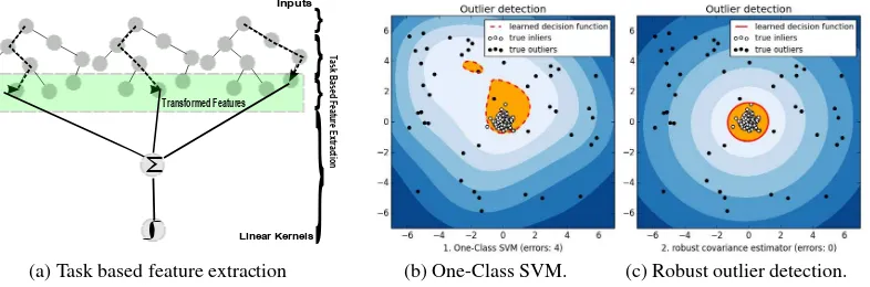
as trajectories generated due to the proliferation of GPS enabled cabs (Zheng et al., 2009) in large metros and increase availability of Wi-Fi hotspots. The computation models needs to learn tra-jectories which can give insight to the behaviours of the users’ for designing future infrastructures. Just as designing a fast pre-fetch cache from web users’ click stream, the tree model needs to capture the branching of the paths by approximating from sparse segments of moving data in motion. When using a tree to repre-sent the trajectories the memory savings could be enormous when compared to the size of the original trajectories due to potential overlaps. Electronically generated streams do not contain labeled data and thus not suitable for supervised algorithms. We propose a powerful overlap function (Prasad et al., 1991) metric to iden-tify the actionable events. The stream pre-processing algorithm is resilient to noise and uses instance based learning and at the same time, works in unsupervised settings (it can have labels). The overlap function determines a proximity count induced by the tree ensembles as shown in Fig 1(a).
We have successfully used Hoeffding bounds to guarantee that the baseline model is within a small probabilityδ from its true mean. We extend the Hoeffding principle to Data Streams (Bifet, 2009a), which have a property of infinite input size. For the in-memory model (Brooks and Iyengar, 1996) (Iyer et al. 2013) (Breiman, 2001) to fit the requirements to handle data in mo-tion, the above rule extraction models needs to address the fol-lowing resource constraints. To store sufficient statistics which are needed to model the stream that are to be held within node splits of the tree in-memory. Hoeffding bounds (Bifet and Kirkby, 2009) states that the estimated mean does not change very much after sufficient samples (n) are seen and this is independent of the distribution. To guarantee sufficient statistics for on-line classifi-cation and to guarantee its true mean we use Hoeffding tree. We also show that Hoeffsing tree is able to compute sufficient statis-tics in memory and achieve a base line accuracy compared to the above two kernel methods tested with large data streams.
In the cases discussed so we assume the datasets have known events even though learning from them efficiently and its scal-ing have been satisfactorily addressed. Still there are rare events which are weekly labelled (due to unbalanced support) as they are buried inside noise and outlier present in large streams. A weekly labelled event (buried events) are illustrated in Fig. 1(b,c) which can occur due to big sample sizes. Data models for large data streams have successfully used to correct such outliers by using Bonferroni principle (Rajaraman and Ullman, 2011) to ad-dress false alarms. We further explore to mine actionable patterns of practical significance using power of SVM in the following ways: (i) One-class SVM for outliers and, (ii) soft-margin SVM for novel patterns.
The rest of the paper is organized into two major sections (i) low-level data-cleaning and (ii) task based feature extraction and statistical model building. Section II, discusses why rare event learning is an NP hard problem and seeks to use existing SVM to solve them. Section III, surveys related work in spatio-temporal domain to explore low-level data-cleaning reliability. Section IV, introduces how algorithms are applied to spatio-temporal data with a task based approach. As we will extend our low-level model with a computation module based on our original overlap function which is non-parametric. In Section V and VI we intro-duces kernel method computations and algorithms to build robust statistical models to deal with dynamic data. Section VII demon-strates the results for spatio-temporal datasets with in-memory models and compares preliminary streaming results with existing standard machine learning libraries. Section VII summaries and concludes the work.
II. RARE EVENT LEARNING
An example from weather dataset contains humidity, rain, tem-perature, and wind to predict the occurrence of fog, a rare event (Garimella and Iyer 2007), when rain attribute value happens to be false. We like to further understand rare events (Lin et al., 2013) and its prediction for label and label-less streams using similarity measures. We already know that non-parametric meth-ods such as k-means clustering needs to know the number of clus-ters a priori. To overcome this limitation we use density based ap-proaches in the feature space, which is explained in Section V. As an introductory example to illustrate this concept by using one-class SVM as illustrated in Fig. 1(b). We estimate the single one-class features and infer the properties of a rare event without assuming the number of clusters a priori. When using pattern recognition using Support Vector Machine (SVM) (Cortes and Vapnik, 1995) to classify rare events we use One-class and soft-margins SVMs
as discussed in this section. The Bonferronis principle states that if the number of events in practice are know to occur can be cal-culated then the outliers can detected and avoided in random data sampling.
Looking at the same problem in terms of a probability density function (pdf), given a set of data embedded in a space, the prob-lem of finding the smallest hypersphere containing a specified non-trivial fraction of the data is unfortunately NP-hard [kernel methods]. Hence, there are no known algorithms to solve this problem exactly. It can, however, be solved exactly for the case when the hypersphere is required to include all of the data. So we first consider the cases when all the data are available.
A. One-Class SVM
When estimating big samples sizes (Lin et al., 2013), one-class SVM can be used in a unsupervised learning setting. We generate two types of random data: one with ’normal’ novel patterns with a fixed meanµand, other with ’abnormal’ novel patterns which are uniformly distributed. The effectiveness of the algorithms is illustrated in Fig. 1(c). The results shows that the SVM is unable to perfectly classify for the underlying unknown distribution as it has some outliers. Use of robust covariance estimator which assumes the data are Gaussian. The plot in Fig. 1(c) has no errors as it applies the Bonferronis principle to further filter the practical limits when applied to big samples.
B. Hinge-loss Cost Function with Soft Margins
When the data is completely random and cannot be completely separated using SVM hyperplane. The hidden events present which may be hard to classify needs and needs to be cross vali-dated by splitting the training set into 80-20% splits and a soft-margin. The soft-margin is an automatic way to rejects a hard to classify sample by using cost function: the learning algorithm needs to balance the ratio of false positives occurring during test-ing (Lin et al., 2013) and help lower them. When a particular pattern has probability close to0.5in the case of a binary classi-fication, then use of soft-margin SVM combined with a penalty function is more efficient to learn the hidden novel patterns we discussed earlier using the complete data. The SVM model can use the soft-margin tuning variablesCandγfor their best fit (Hu and Hao, 2012; Iyer et al., 2012). The key is to tune the soft-margin hyperplane with the variable (ξi) for standard SVM hard hyperplane (Cortes and Vapnik, 1995). SVM equation as shown below.
yi(xTiw+b)≥1yiǫ{−1,1} We define a convex cost-function such that
yi(xTiw+b)≥1−ξiξi≥0
The new estimate using reject option further helps to disambiguate hard to classify samples.
How to compute and estimate large sensor data streams to mine rare events:
• Feature Engineering - ”Data driven learning”
– Instance based label-less feature task-based induction
• Streams Models - ”Data in motion”
– Efficient in-memory sufficient statistics
– One-class novel pattern detector using Bonferroni cor-rection
– Soft margin SVM using loss function to find hard to classify patterns
Current work focuses on feature extraction using explicit learning algorithms. Events can be learned using labels or sometimes hard to classify datasets. SVM based kernels can disambiguate hard to classify datasets using soft-margins. Most of the learning algo-rithms still have the training phase which make them unsuitable for real-time analytics. In the domain of sensor networks, dis-tributed measurements have been successfully calibrated (Prasad et al., 1991) with fault tolerant (Prasad et al., 1993) algorithms to avoid false alarms. The techniques used in feature extraction and real-time fault tolerance does not address rare event learning di-rectly. As rare events can be patterns, which may not necessarily be induced by basic feature occurring in the dataset. The ability to detect rare events is of at most importance, and needs the ability to predict such occurrence without training from past data. The proposed AI based rule learning technique allows to bridge the gap between feature extraction and real-time rare event mining.
III. RELATED WORK
It is a known fact that when dealing with big samples the p-value (Lin et al., 2013) linearly decreases causing false events detection even though they are not significant. In a similar way the learn-ing algorithms have to deal with ”curse of dimensionally” with respect to attributes and ”curse of support” (Kar and Karnick., 2012) when determining support vectors using SVMs. There is a related problem of missing values in the dataset and how the in-memory model addresses it for a particular task. The work by Vens and Costa (Vens and Costa., 2011) on Random Forest a task based feature induction, deals with statistical and missing value sub-problems. A similar work by Bach and Jordan (Bach and Jordan., 2005) to compute a predictive low-rank decomposition for task based feature induction using kernel methods have ad-dressed the same issue. In this work we use both methodologies to study the statistical properties and the quality of data related to the fitness needed in mobile data driven applications.
The parallel computation of large tree ensembles has been re-cently addressed by Breiman and Adele Cutler (Liaw and Wiener., 2002). Which combines individual tree representation (Chang et al., 2006) with a distributed feature table (big-memory scaling). New frameworks such as R Programming Studio, Mapreduce, and Spark MLLib, now support distributed processing just be-yond< key, val >pairs. The pre-processing language seman-tics support in the latest version of Spark further allows efficient feature extraction in retime. Which enables existing batch al-gorithm to be ported to real-time sensor data stream environment effortlessly.
When using kernel matrix to approximate higher-dimensional fea-ture space to lower-dimension space, further allows to address the huge number of SV’s. The optimization in (Kar and Karnick., 2012) helps to linearly scale (refer to detailed proof) with the size of input. The scalability of computation model is fast but it does not help the predictive performance when features are indepen-dent of their attributes. When modeling data of a user’s trajectory or other forms of synthetic data, the features cannot be general-ized by using the basic patterns and may not form regular clusters. So one cannot use non-parametric clustering when the number of clusters are not known a priori. So we argue the use of explicit overlap function (Prasad et al., 1991) feature induction in these
cases works well. We further extend sensor data streams for fast predictive overlap models which can handle real-time constrains.
On-line processing of noisy sensor measurements has been ex-tended to distributed framework by Brooks-Iyengar (Brooks and Iyengar 1996). This seminal work balances precision and accu-racy to estimate the non-faulty (Iyer et al., 2008) sensor’s con-fidence intervals. Real-time algorithm has been extended us-ing Byzantine fault-tolerance principle to mitigate faulty sensors (Brooks and Iyengar., 1996), which are likely to trigger false alarms. The power-aware distributed computation is due to its simplicity and the protocol keeps communication overhead to a minimum using in-network processing and with minimum cen-tralized coordination.
IV. AUTOMATIC RULE EXTRACTION
Computational data sciences has massive amounts of datasets gen-erated from remote sensing and, periodic stream updates from several sites spread across many geographical regions. Much of the publicly available datasets have not been analyzed for the lack of computationally viable algorithms. Stream analytics cannot scale due to the following reasons: the known p-value statistical problem (Lin2013c) with large scale datasets; the statistical sig-nificance of a common feature increases linearly with number of samples.
A. Calculating Higher Order Side Information
In this paper we are not only interested in rare event prediction but also the temporal rules (slow moving in time) which attributes to it. Important patterns occurring many times in the data if there is enough support then it becomes a rule. Due to this large size datasets needs to estimate rare events in practice differently. One such estimation was suggested by the Bonferronis Principle. Which states that models ability to mine data for features that are not sufficiently rare in practice. Scientist in this domain have used raw sensor attributes which when combined with learned coefficients help to form linear ranking index functions such as Fire Weather Index (FWI) estimation. Using FWI ranking the streams from the weather model can track the time-series sensor stream and predict rare events before than can happen. Due to the number of datasets available for rare events being few for train-ing, we propose an automatic methods to detect such events in a timely fashion. When mining massive datasets the rule extrac-tor is a correlated side-information (Iyer et al., 2013b) present in the target concepts. Some of the feature extraction are discussed with sensor data (Table I) and ground truth examples (Zheng et al., 2009).
We generalize a predictive functions which has the following rules:
Descriptive inputsattt1,attt2→side-information
The predictive rule suggests that the inputs of the dataset are highly correlated to a few target attributes, which then uses as ob-jective measures by tracking the side-information - especially in the case of unlabeled streams. As an example we use the Landsat dataset (Newman and Asuncion 2007) from University of Irvine, Machine learning repository. Landsat dataset attributes have the following attributes: channel-R; channel-G; Channel-invisible1, Channel-invisible1. For example, the extracted rule for our e.g. dataset is:
channel-R; channel-G→channelinvisible1, channelinvisible2
∫
(a) Task based feature extraction (b) One-Class SVM. (c) Robust outlier detection.
Fig. 1 Learning methods using linear and non-linear feature space.
2007) and the observed values of invisible channels, because the measured scenes are one and the same for the visible band and the satellites invisible band. There was no significant deviation in the normalized Root Mean Square Error (RMSE) values during training and testing, suggesting the use of the side-information are ideal in practice, when using regression trees.
The side-information concept can be extended (Iyer et al., 2013b) to rare events such as forest fire by computing the temporal FWI of that region. The above rule can then be written for FWI (Iyer and Iyengar et al., 2011) as:
temp1, humidity1, wind1, precipitation1 →FWI scalar (0-80)
B. Performing Clustering Based On Data Cleaning Trees
The ensemble model which is illustrated in Fig. 1(a) uses Ran-dom Forest where the node splits are based on clustering target variables. The target variables help in finding unique clusters as discussed in this section. The prototype function (Vens and Costa 2011) used for clustering and node splitting helps to estimate the model density thresholds for the current window. The induction of such a tree with actionable events results in extracting their local temporal rules for further labeling and on-line event dash boarding.
V. TASK BASED DISTRIBUTED FEATURE ENGINEERING
Feature engineering as a domain, focuses on learning from data streams without a priori knowledge of the underlying process or the number of clusters. Source of the generating process are un-known and random and due to their high variance its validation can be only done solely by use of ground truth. Ground truth can be in the form of past events recorded by weather station logs and verifiable timestamps overlapping the same period as of the train-ing dataset. Assumtrain-ing that rare events are present in the data we focus on various task-based feature induction as described in Fig. 1(a). We discuss the advantages of task based learning compared to learning the kernel functions and how it handles missing val-ues. The common metric used by the learning functions are non-parametric (distance and similarity) induced in the feature space, but we are interested in learning the fusion of spatio-temporal features. The task based explicit feature metric representation has other advantages. The computational advantage is that it does not need to learn the pair-wise distance and need not store quadruple amount of information such as the Gram Matrix. A tree based representation naturally allows to deal with missing values, com-pared to existing statistical methods.
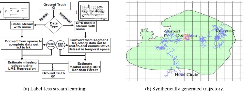
We illustrate the stream model for both cases using static data-driven algorithms and mobile wireless application testbed as shown in Fig. 2(a). There are two forms of stream quality (Iyer et al., 2013a) non-parametric ranking for random streams which are shown in Fig. 2: kappa score for missing values and, finding actionable events of interest. Kappa score (Iyer 2013a) helps to compare how the learning algorithm perform using euclidean dis-tance measure when dealing with spatial measurement. For tem-poral end-to-end trajectory streams, an explicit similarity mea-sure is learned from Random Forest ensemble as shown in Fig 1(a). Which allows to learn similar trajectories during model training. Both these methods are cross-validated by the ground truth for selecting and refining the models for noisy, static and mobile streams. When growing the Random Forest ensembles the tree splitting at the root node is selected along one of thesev attributes to minimize the number of misclassified training points if a majority vote is used in each node. The procedure is repeated until every node is pure and assumes the following assumptions such asn training samples and the samples are saved and can be read back many times. The current assumptions cannot be applied for real-time algorithms which cannot store stream sam-ples and read the samsam-ples only once. Comparing the real-time Brooks-Iyengar’s algorithm the metric used for parameters’ con-fidence interval approximation are the weighted average of pre-cision and its accuracy (Brooks and Iyengar 1996) over all the sensor measurements. As our task based distributed feature en-gineering needs to scale in a real-time window. The distributed framework need to extend the current feature splitting method-ology to an iterative learning model, which can handle data in motion while computing in-memory.
Summary of the iterative stream learning model:
• Uses Hoeffding bounds for statistical sampling
• Uses task-induced similarity measure metric
• Handles missing value by randomization
• Distributed in-memory features representation using big-table
• Real-time computation guarantees to process fast streams
(a) Label-less stream learning. (b) Synthetically generated trajectory.
Fig. 2 The prototype of rare event learning functions using distance and similarity of sensor streams produced by trajectory being cross-validated with ground truth for stream quality.
two-dimensional GPS datasets provided high accuracy in predict-ing actionable events with large datasets. Hoeffdpredict-ing tree and AI (Garimella and Iyer 2007) based ANOVA kernel computational model optimize resource requirements by one-tenth of other well proven models such as Naive Bayes and non-linear kernels.
VI. METHOD
Lower-level sensor measurements task are prone to errors due to noise and faulty (Iyer et al., 2008) sensors. Incorrect results can be obtained as the upper level Gram Matrix relies on tuning few parameters. Higher level data mining tasks should be descrip-tive that summarizes the underlying relationships in data. To de-sign a data-driven application the low-level should be task driven that is independently supported by higher-level information. Our higher-order feature induction approach uses learning as follows: ensemble overlap similarity, Gram matrix using kernel methods, and moving window using an iterative Hoeffding tree model. Re-lated work shows that kernel methods have higher predictive per-formance but does not allow to intuitively understand the rules extracted from them given the original input space. As we are analyzing data which has temporal attributes it is equally im-portant to extract the thresholds which support them. Due to mobility based location context requirements, our emphasis is based on natural or explicit rule learning and does not rely on high-dimensional Gram matrix. Once the rule extraction process synchronizes with the low-level mining task, one can compare its performance over a moving window using on-line Hoeffding tree. The implementation methods discussed below addresses the following memory requirements for any data stream type. How learning natural rules from data can be learned in a task driven model.
A. Algorithm
Real-time algorithms needs to maintain sufficient statistics and the tree structure in memory. The incremental tree updates due to the changing statistics are performed by splitting using the best attribute. When referring to kernel methods anN×N Gram matrix or an optimized lower rank is stored in memory.
1) Quallity of Data and Big Matrix Representation The use of tree structure allows efficient in-memory model and at the same time we like to extend the idea of instance based feature induction in our mobile applications. Random Forest ensemble builds many trees which prevents model over-fitting. The imple-mentation of the distributed big-table (Chang et al., 2006)is by
allowing the ensemble growth of the current working set to be more than the available fast memory. Internally the big table is implement as a shared distributed table across worker nodes. Af-ter the ensemble parameAf-ters are tuned and built with sufficient number of trees then the model is tested. We use the training set (n) and the out-of-bag samples together, and traverse down the trees (t) taking one input sample at a time. In the case of similar samples they will end up in the same terminal nodes (m-leafs) usingn(tlgm)steps. For those cases the model increases the proximity count by one. To get a number between (0-1), the model divides the proximity counts for each case by the number of trees in the ensemble. The elements in the big-matrix will esti-mate the number of times instances [m and n] end up in the same node. This sparse measure is useful for upper-level trajectory learning as shown in Fig. 2(b)and other higher task based rule ex-tractions from random and synthetic datasets. Computation over-head for the calculation of Gram matrix can have a worst case of N×N. The proximity computation of a Random Forest ensem-ble is always efficient. The framework can handle any number of attributes when performing proximity calculation in parallel with less than ten classes. We show the worst caseN×Ncomplexity of calculating the primal Gram matrix can be efficiently com-puted using via its duel representation. The data-cleaning duel framework’s computation are only dependent on the number of spatio-temporal features and is given byO(N l)(Shawe-Taylor and Cristianini, 2004) wherelare linearly independent attributes found using kernel transforms.
2) Data in Motion When estimating events from big sample data which can run into 10,000 or more observations. The p-value is inversely proportional to number of samples, the value goes quickly to zero asnincreases. Relying on p-value estimation alone cannot find events of practical significance we use a con-fidence parameterδto determine the node splits. Due to model building with fixed size datasets is not possible with limited mem-ory, we propose a real-time windowed data stream model us-ing Hoeffdus-ing bounds (similar approach to Brook-Iyengar algo-rithm):
1. Data Streams cannot be stored and an emphasis of in-memory model is assumed to have low processing latency
2. Sufficient statistics are kept which are essentially a summary of the data and requires very small memory.
Constraints (1) and (2) addresses the in-memory requirements of the data mining algorithm. The constrain (3) for recalculating the statistical summaries uses a sliding window concept, by which the last W items are used in the model which have arrived. If the size of W is moderate then the first two constraints (1) and (2) are satisfied. The rate of change of spatio-temporal events determine the optimum size of W. There are two case for selection of W: (i) the rate of change is small compared to the size of W and (ii) the data in motion can be drastic but the drastic changes are often greater than W. The optimal W will vary on the accuracy of the sensors and the higher level streaming application.
The in-memory iterative model uses a windowWwhich is parti-tioned intoW0·W1with lengthsn0, n1, such thatn=n0+n1.
To determine sufficient statistics for our iterative model we de-fineǫcutwhich minimizes the error(1−δ). To further guarantee real-time performance we rely on harmonic mean defined by:
m= 1 1
There are two cases which can be used for performance guaran-tees that estimate the change in distribution using a statistical test.
Theorem 1. The performance of our model depends upon on event rate processing. The data stream model performs in incre-mental time steps and we have:
1. False positive rate bounds. If the optimal window size is chosen for the Data Stream application then µt remains constant within the windowsW. The probability that AD-WIN will shrink the windows at this time step is at mostδ. 2. False negative rate bounds. When the optimal window size
W is not known a priori for the Data Stream applications some events may be ignored due to the overlapping settings
µ0−µ1 >2ǫcut. Then with probability1−δ,W shrinks toW1in the next time step.
Proof. Assureµw0=µw1=µw, we show that for any partition
W asW0W1we have probability δnthat ADWIN will decide to
shrinkWtoW1, or equivalently.
P r[|µw1−µw0| ≥ǫcut≤δ/n]
Since there are at mostnpartitionsW0W1, the claim follows by
the union bound. For every real numberk∈(0,1),|µw1−µw0≥
ǫcut|can be decomposed as
P r[|µw1−µw0| ≥ǫcut≤P r[|µw1−µw|
≥kǫcut] +P r[|µw1−µw|
≥(1−k)ǫcut] Applying the Hoeffding bound, we have then
P r[|µw1−µw0| ≥ǫcut≤2exp(−2(kǫcut)2n0)
+2exp(−2((1−k)ǫcut)2n1)
Minimizing the sum, we choose the the value ofkthat makes both probabilities equal.
Therefore, to satisfy we have
P r[|µw1−µw0| ≥ǫcut]≤ δ
hypothesis. Using the Hoeffding bound, we have then
P r[|µwˆ0−µwˆ1| ≥ǫcut]≤2exp(−2(kǫcut)2n0)
+2exp(−2((1−k)ǫcut)2n1
Now, choosekas before to make both terms equal. By the calcu-lations in Part 1 we have
P r[|µwˆ0−µwˆ1| ≥ǫcut]≤4exp(2mǫ2cut)≤ δ
n ≤δ as desired.
Algorithm 1Adaptive Windowing Algorithm
1: procedureADWIN(a, b) ⊲The g.c.d. of a and b 2: fort >0do
3: Do W ←W∪xi
4: repeatDrop elements from the tail of W 5: until|µwˆ0−µwiˆ | ≤ǫcut holds
this technique for the representing the model does need a train-ing phase; instead it learns incrementally and can be used to test new samples at any given time to keep up with high speed of stream processing. Hoeffding bound states that the true value of the meanµ, of a random variable of rangeR, can be practically approximated for big samples afternindependent observations by more than (with a low probability of error):
ǫ= r
R2lg(1/δ)
2n
The estimation using this bound is useful as it is independent of the distribution. Maintaining sufficient statistics are explained in
Algorithm 2Hoeffding tree induction algorithm
1: fortraining examplesdo
2: Sort example into leaflusing HT 3: Update sufficient statistics inl
4: Incrementnl, the number of examples seen atl
5: ifnlmodnmin = 0and examples seen at l not all of same classthen
6: ComputeGl(Xi)for each attribute 7: LetXabe attribute with highestGl¯ 8: LetXbbe attribute with second-highestGl¯ 9: Compute Hoeffding boundǫ=
q
R2lg(1/δ)
2n 10: end if
11: ifXa6=X0and( ¯GlXa−Gl(Xb)¯ > ǫorǫ < τ then
12: Replacelwith an internal node that splits onXa
13: forbranches of the splitdo
14: Add a new leaf with initialized sufficient statistics 15: end for
16: end if 17:
18: end for
(line 4-6) of Algorithm 1. Node splitting and how the tree grows are show in line (12-15) in Algorithm. The Hoeffding bounds allows to compute the true mean with in a reasonable margin of error. The growth of the Hoeffding tree can be show in Algorithm 1, is compatible [email protected](Lin et al., 2013) which is desired for big sample data sizes.
Algorithm 3Hoeffding Window Tree(Streamδ)
1: procedureEUCLID(a, b) ⊲
2: Let HT be a tree with a single leaf(root) 3: Init estimatorsAijkat root
4: forexample(x,y) in Streamdo
5: HWTreeGrow((x,y),HT,δ)
6: end for 7: end procedure
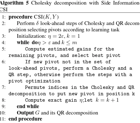
3) Cholesky Decomposition with Task based Side Informa-tion - CSI Kernel based data driven learning has become popu-lar as there are publicly available software libraries which support to solve complex matrix multiplication, pseudo inverse and con-vex optimizations needed in vector modeling (Kar and Karnick., 2012). One of the popular forms of factorization is Cholesky decomposition (Bach and Jordan., 2005). Since the Cholesky de-composition is unique, performing a Cholesky dede-composition of the kernel matrix is equivalent to performing GramSchmidt or-thonormalisation in the feature space, and hence we can view Cholesky decomposition as the dual implementation of the Gram-Schmidt orthonormalisation. The normal Gram matrix obtained from this is very large and in the order ofN2. The general
opti-mization does not include side information which are in the form of class labels or response variables. Our previous discussion on using a sparse representation instead of full Gram matrix (Bach and Jordan., 2005) can be realized by this method. While the optimizatio step pivots are generated during factorization an ad-ditional optimizations is used by CSI to include the remaining la-bel information. Which allows to generate sparse and most of the time lower ranked matrices compared to the the general Cholesky methods. CSI optimization methods allows to reduce size of the final matrix allowing fast in-memory kernel models without loss of prediction accuracy. Similar to our previous approach of using
Algorithm 4Hoeffding Window Tree(Streamδ) 1: procedureHWTREEGROW(((x,y),HT,δ)) 2: Sort(x, y)to leaf l using HT
3: Update estimatorsAijk
4: at leaf l and nodes traversed in the sort 5: iflinTaltthen
6: HWTreeGrow((x,y),Talt, δ) 7: end if
8: Compute G for each attribute 9: Evaluate condition for splitting leafl 10: if(Best Attr.)-G(2nd best)> ǫ(δ′, ...)then
11: then Split leaf on best attribute
12: end if
13: foreach branch of the splitdo
14: Start new leaf
15: and initialize estimators 16: end for
17: ifif one change detector has detected changethen
18: Create an alternate subtree Talt at leaf
l if there is none
19: end if
20: ifexisting alternate treeTaltis more accuratethen
21: then replace current node l with
alternate tree Talt
22: end if 23: end procedure
task based Random Forest metric representation, we employ task based optimization to kernel matrix decomposition as described in CSI (Bach and Jordan., 2005) Algorithm 4. As previous dis-cussed the kernel matrix are huge (Chang et al., 2006) and in the order ofN2for real-time processing. To reduce the rank of the kernel matrix we use its labels (side-information) to mitigate piv-ots (▽) used during matrix factorization. The spatial feature and its residual characteristic of the significant Eigen values (λ) and its following Eigen vectors (ν) are studied, the final rank obtained is always lower than theN2Gram matrix. Lines 5-9 in Algorithm
VII. EXPERIMENTS ON UCI AND MSR DATASETS
The spatio-temporal datasets used in testing included forest cover (UCI), Statlog (UCI), and Geolife (Zheng et al., 2009) training and testing sets. We study the two task induced in-memory mod-els: (i) QoD and explicit rule proximity matrix learning with-out kernel (bigrf-Table), and (ii) kernelized implementation in R based on labels (CSI-Kernel class). The performance of the predictive models are compared in three different memory scales (shown in x-axis of Fig 3): temporal windows in real-time (samples-per-sec), Original input space (Batch)(R2), andN×Ninduced
big-table feature space(Rd)(see Fig 3.)
A. Estimating Events Using Hoeffding Bounds for Big Sam-ple - Real Variables
When estimating big samples the underlying source can be one of the following distributions:
• Normal
• Uniform
Algorithm 5 Cholesky decomposition with Side Information-CSI
1: procedureCSI(K, Y)
2: Performδlook-ahead steps of Cholesky and QR decom-position selecting pivots according to learning task
3: Initialization:η= 2ε,k= 1 4: while doη > εandk≤m
5: Compute estimated gains for the
remaining pivots, and select best pivot
6: If new pivot not in the set of
look-ahead pivots, perform a Cholesky and a QR step, otherwise perform the steps with a pivot optimization
7: Permute indices in the Cholesky and QR
decomposition to put new pivot in position k
8: Compute exact gain η;let k=k+ 1
9: end while
10: OutputGand its QR decomposition 11: end procedure
The accuracy of the ensemble model cannot be based on p-value alone as discussed in earlier sections. We introduce an reliabil-ity factor (Iyer2009b) which is used as a confidence measure to further distinguish the best feature to split on at the nodes. The sufficient statistics used by the in-memory model for prediction is based on Hoeffding bounds whereδ≥ǫ(statistical significance).
δ=
1) Performance in Real-Time- Using Hoeffding bounds To simulate a huge live streams we used the forest cover type dataset (Newman and Asuncion., 2007b), which has over 581,012 la-beled samples. The predictive model builds a Hoeffding tree with 155 leafs nodes. Which took 12.69 seconds to build the tree in memory with a node splitting probability [email protected]. The Ho-effding tree uses a very fast decision tree and closely approxi-mates a full fledged decision tree. The estimated reduction of tree size from the original 53,904 leafs used by Random Forest classifier compared to 155 leafs used by Hoeffding tree. This fast decision tree implementation with incremental learning performs with a baseline accuracy of 79.5%.
Sensors S1 S2 S3 S4
Observed 4.7±2.0 1.6±1.6 3.0±1.5 1.8±1.0
TABLE I A typical sensor dataset.
S1 S2 S3 S4 Overlap
S1 1 0 1 1 0.66
S2 0 0 2 1 1
S3 1 1 0 1 1
S4 1 1 1 0 1
TABLE II Proximity counts after addingS4 (good sensor) the
ensemble overlap estimation now changesS1to tamely faulty.
B. Estimating Events Using Hoeffding Bounds Random Vari-ables - Explicit Lower Dimension Representation
When mapping higher dimension space to an approximate linear lower dimension space, we use the following conversion:
• Euclidean distance
• Proximity distance
Optimization accuracy for linear case is:
sup|< Z(x), Z(y)−K(x, y)>| ≤ǫ
1) Explicit Rule Extraction (Non-Gram matrix) in one di-mension -R A typical sensor measurement with an average and range that are provided as an base case example in Fig. 1. Using our proposed explicit feature metric which can be scaled between[0,1]. This allows a uniform metric for all applications and to compare events of interest in any domain. In the exam-ple of four sensors we initially take three out of four to form an ensemble feature matrix. The matrix uses our proposed explicit feature representation as shown in this section. As shown in Fig. 3 (and tables)S1 and S3 fall into the same terminal node and
their proximity count is incremented by one. Table I shows the overlapping rules on the right show the overlapped measure of reliability ofS1−S3combined. If we use fuzzy interval
defini-tion of sensors to represent the varying levels of overlap then we represent its reliability by:
• Non faulty (= 1)
• Tamely faulty (≥0.5)
• Widely faulty (≤0.5)
Applying the rules to our dataset we findS2andS3are non faulty
(as illustrated in table) as they have the maximum overlapping count. At the same timeS3andS2is tamely faulty asS2is
in-clusive ofS3. The higher level application can now rely on
mea-surements fromS2andS3for its precision and range accuracy.
To further see the ensemble optimization we introduceS4 and
create the new feature matrix as formed in Table II. Reading from the data in the overlap column we see thatS4 has a maximum
overlap of 1. The addition does not have any effect onS1. The
accuracy of the random subspace learned from the trees include S4as it has a narrow range compared to all others. The accuracy
Sensors S1 S2 S3
1 2.7 0 1.5
2 4.7 1.6 3.0
3 6.7 3.2 4.5
... ... ... ...
S1,S 3
S1 S2 S3 Overlap
S1 1 0 2 0.67
S2 0 0 3 1
S3 1 2 0 1
Fig. 3S1&S3end up in the same terminal node. The Big-Table proximity count is incremented by 1. (The color metric in the overlap
columns specifies quality of data: Green=non faulty; Blue= tamely faulty; Red=widely faulty)
BUS CAR WALK Overlap
BUS 488 0 76 0.135
CAR 0 516 1 0.001
WALK 133 1 294 0.313
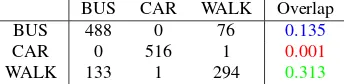
TABLE III Feature induced matrix using two dimensional datasets.
2) Explicit Rule Extraction (Non-Gram Matrix) in two di-mension -R2 Experiments are conducted Using the Geolife
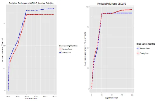
trajectory dataset similar to the one-dimensional case discussed as the base case example. The explicit learning algorithms use a tree structure to learn the user’s trajectories generated by mobility models of car, walking and riding bus. The matrix representation of the feature space shows that the mobile user’s walking class has the highest information gain as marked (green) in Table III. The predictive peak performance of bigrf-table is 96% for an en-semble size of 100 trees as shown in Fig. 5, when compared to the real-time streaming model. The added memory overhead of using aN×N in the two-dimensional case is solved by using distributed shared configuration across multiple nodes of a clus-ter.
C. Estimating Events Using Hoeffding Bounds for Kernel Variables - Curse of Support
When dealing with support vector machine to transform non-linear relations to non-linear space we use the following kernels:
• ANOVA kernelk(x;x′) =P
1≤i1...<iD≤N
QD
d=1k(xid, x ′
id)
• Bassel Kernelk(x;x′) = (−Besseln
y+1ρ||x−x ′
||)
• Radial Basis Kernelk(x;x′) =exp(−ρ||x−x′||2
)
• Laplace Kernelk(x;x′) =exp(−ρ||x−x′||)
Optimization accuracy for non-linear case is:
sup|K(x, y)| ≤ǫ
1) Data Representation Using Gram Matrix with Side Infor-mation Optimization - FRd For computational comparison, we perform feature space analysis using the Incomplete Cholesky (CSI) R package. The task based optimization uses pivoting to
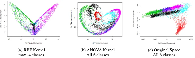
reduces the original [4434x4434] matrix. The final feature ma-trix rank is reduced from 4437 to 20 as show in Table IV. The lower rank outcome is based on the type of features induced us-ing the kernel functions. ANOVA kernel uses the least number of samples and at the same time has superior prediction accuracy. The rest of the kernels RBF, Laplace and Bassel have comparable accuracies but the computation is5×slower due to large matrix ranks. Further using visualization and projection as shown in Fig. 4. (Scholkopf et al., 1999) reveals that ANOVA kernel is able to induce higher-order features (up to 20) to separate all the six cat-egories. This is due to ANOVA being able to learn statistical similarities from subspaces and represent them efficiently as fac-tors. Earlier results verifies from section IV on side-information using associates rules for the same dataset that the attributes are statistically correlated.
The same experiments are repeated without PCA like optimiza-tion and using the kernels directly with the input datasets. The following results for the non-optimized Gram matrix are shown in Table V. The overall reduction is accuracy is by 10%.
2) Data Representation UsingN×N Gram Matrix - with No Memory Optimization The standard kernels: ANOVA, Gaus-sian RBF and linear SVMs are used with full rank matrices (i.e. without memory optimization). The non-optimized model’s ac-curacies are moderate to base line variability, when compared to kernels with in-memory optimization. The comparative results are illustrated in the Fig. 4., ANOVA-kernel has a peak perfor-mance of 89.56% is significantly lower than the task based ap-proach. The kernel KSVM R package (Karatzoglou et al., 2004) allows to tune the SVM (Blanchard et al., 2004) soft margin pa-rametersCandγby use of cross-validation. The higher theC the better would be the fit (see Section 2), but it may not general-ize well. Using the cross-validation techniques discussed above, we arrive at d=2,sigma=0.015,C=50, when using cross-validation (cross=4) for the spatio-temporal example UCI dataset (Newman and Asucion., 2007).
TABLE IV Reconstruction Error: Results for the UCI-Landsat dataset when pre-processing features with statistical properties of kernels (included Incomplete-Cholesky).Configuration:Intel i5-2435M Processor, 2.40GHz; 4GB DDR3. The timings included show feature extraction during pre-processing. Side-Info column indicates if it is supervised or unsupervised learning.
Pivot election Training Accuracy Rank SV Time (Batch in sec.) Side-Info.
ANOVA kernel 89.6% 20 20 40 Y
Laplace kernel 86.5% 100 1489 120 Y
Bassel kernel 86.4% 100 1488 120 Y
RBF kernel 78.6% 100 1636 120 Y
Inchol RBF - 3067 - - N
TABLE V Prediction Error: Results for the UCI-Landsat dataset when post-processing to predict or categorize the datasets using unknown test samples. The timings included show training time during learning the models.
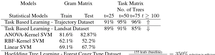
Models Gram Matrix Task Matrix
No. of Trees Statistical Models Train Test t=25 t=50 t=75t≥100 Task Based Learning - Trajectory Dataset 91% 95% 96% ⇑ Task Based Learning - Landsat Dataset 89% 91% 85% ⇓ ANOVA-Kernel SVM 81.6% 82.87%
RBF-Kernel SVM 62.1% 52.2%
Linear SVM 69.1% 67.7%
Hoefdding Tree Learning - Forest Cover Type Dataset 53904155 leafs (baseline)leafs (original RF) = 350%reduction in sufficient stats.
The ensemble based rfBig explicit deep feature engineering frame-work performs significantly well for the synthetic datasets such as trajectories. The popularity of distance based kernel method shows how higher-order features helps to better predictive per-formance, without knowing a priori the underlying distribution, specially with few number of training data.
VIII. CONCLUSION
In this work we have extended an existing real-time sensor net-work algorithm using Hoeffding bounds to learn rare events of practical significance which can be applied to any stream distri-bution. The rare event feature learning which are computation-ally expensive have been adapted for resource constrained real-time streaming needs. The enhancements distinguishes the im-pact on model performance which sometimes can be biased due to the datasets. The spario-temporal concepts learned shows that explicit rule learning has many advantages and can significantly increase performance when used with mobile trajectories. On the other hand when learning the kernel function and its Gram matrix, and using far more induced features helps the model to predict with higher accuracy. The use of spatio-temporal datasets brings out the art of pattern recognition and AI to life. The task based approach when applied to explicit and kernel based pre-diction has shown improved accuracy compared to earlier kernel versions. This AI framework’s enhancements will help develop geo-spatial applications which can reliably and efficiently find actionable events from satellite imagery. The learning of stream uses a non-parametric approach for outliers detection in time se-ries streams and, a task based approach to improve QoD.
ACKNOWLEDGEMENT
The project was supported by HRD/DHS/AFRL/Microsoft Azure for Research programs. This work was supported by the follow-ing grants: NSF grant HRD-1137466, DHS grants 2011-ST-062-0000046, 2010-ST-062-0000041, 2014-ST-062-000059, AFRL Re-search Collaboration Program Contract FA8650-13-C-5800 and Microsoft Azure Sponsorship awardd2354557/66de/4389/9744/
2e5fab48f38ffor 2015. Also, the mentoring effort by Shailesh
Kumar at Google is much appreciated. The mathematical frame-work for the computation module and earlier research in section V was based on the motivation of CVIT, Hyderabad. The au-thors would like to thank Anoop Namboodiri, C. V. Jawahar, P. J. Narayanan, Kannan Srinathan and Rama Murthy for their help in the submission of the paper (Garimella and Iyer., 2007) which helped the formulation of the dual for our overlap functions.
REFERENCES
Agrawal, R., Imieli, T., Swami, A., 1993. Mining Association Rules Between Sets of Items in Large Databases. SIGMOD Rec. 22, 2 (June 1993), 207216. DOI:http://dx.doi.org/10.1145/ 170036.170072
Bifet, A., Kirkby, R., 2009. DATA STREAM MINING A Practi-cal Approach. University of Waikato, New Zealand (2009).
Brooks, R.R., Iyengar, S.S., 1996. Robust Distributed Computing and Sensing Algorithm. IEEE Computer 29, 6 (June 1996), 5360.
DOI:http://dx.doi.org/10.1109/2.507632
Breiman, L., 2001. Random Forests. Mach. Learn. 45, 1 (Oct. 2001), 532.DOI:http://dx.doi.org/10.1023/A:1010933404324
Bach, F.R., Jordan, M.I., 2005. Predictive Low-rank Decompo-sition for Kernel Methods. In Proceedings of the 22Nd Interna-tional Conference on Machine Learning (ICML 05). ACM, New York, NY, USA, 3340. DOI:http://dx.doi.org/10.1145/ 1102351.1102356
Blanchard, G, Bousquet, O., Massart, P., 2004. Statistical perfor-mance of Support Vector Machines. Technical Report.
Cortes, C., Vapnik, V., 1995. Support-Vector Networks. Machine Learning 20, 3 (1995), 273297. DOI:http://dx.doi.org/10. 1023/A:1022627411411
(a) RBF Kernel. (b) ANOVA Kernel. (c) Original Space.
max. 4 classes. All 6 classes. All 6 classes.
Fig. 4 Random project methods for kernel learning: PCA of stream data taken from four Statlog channels to detect six soil types. Soil types are separated using higher-order statistical properties in (a),(b) and (c). (a and b) are higher-order statistics while (c) are present in the original dataset. The hyperplane boundaries in (a) are able to separate all the six classes while in (b) a maximum of five are uniquely separable.
A Distributed Storage System for Structured Data. In Proceed-ings of the 7th USENIX Symposium on Operating Systems De-sign and Implementation - Volume 7 (OSDI 06). USENIX As-sociation, Berkeley, CA, USA, 1515. http://dl.acm.org/ citation.cfm?id=1267308.1267323
Garimella, R.M., Iyer, V., 2007. Distributed Wireless Sensor Net-work Architecture: Fuzzy Logic Based Sensor Fusion. In New Dimensions in Fuzzy Logic and Related Technologies. Proceed-ings of the 5th EUSFLAT Conference, Ostrava, Czech Repub-lic, September 11-14, 2007, Volume 2: Regular Sessions. 7178.
http://www.eusflat.org/proceedings/EUSFLAT2007/papers/ IyerVasanth(24).pdf
Hu, F., Hao, Q., 2012. Intelligent sensor networks: the integra-tion of sensor networks, signal processing and machine learning. CRC Press, Hoboken, NJ.
Iyer, V., Rama Murthy, G., Srinivas, M. B., 2008. Min Loading Max Reusability Fusion Classifiers for Sensor Data Model Au-gust 2008 SENSORCOMM 08: Proceedings of the 2008 Second International Conference on Sensor Technologies and Applica-tions.
Iyer, V., Iyengar, S.S., 2011. Modeling Unreliable Data and Sen-sors: Using F-measure Attribute Performance with Test Samples from Low-Cost Sensors. 2011 IEEE 13th International Confer-ence on Data Mining Workshops 0 (2011), 1522.
Iyer, V., Iyengar, S.S., Pissinou, N., Ren, S. 2013a. SPOTLESS: Similarity Patterns Of Trajectories in Label-lESS Sensor Streams, The 5th International Workshop on Information Quality and Qual-ity of Service for Pervasive Computing 2013, San Diego, CA.
Iyer, V., 2013b. Ensemble Stream Model for Data-cleaning in Sensor Networks. Ph.D. Dissertation. Florida International Uni-versity, Miami, FL. ProQuest ETD Collection for FIU. Paper AAI3608724.
Iyer, V, Iyengar, S.S., Pissinou, N., 2012. Intelligent sensor net-works: the integration of sensor networks, signal processing and machine learning, Chapter Modeling Unreliable Data and Sen-sors: Using Event Log Performance and F-Measure Attribute Se-lection;. In Hu and Hao [2012].
Kar, P., Karnick, H., 2012. Random Feature Maps for Dot Prod-uct Kernels. CoRR abs/1201.6530 (2012).http://arxiv.org/ abs/1201.6530
Karatzoglou, A., Smola, A., Hornik, K., Zeileis, A., 2004. kern-lab An S4 Package for Kernel Methods in R. Journal of Statisti-cal Software 11, 9 (2004), 120.http://www.jstatsoft.org/ v11/i09/
Lin, M., Lucas, H.C. Jr., Shmueli, G. 2013. Research Commen-tary - Too Big to Fail: Large Samples and the p-Value Problem. Information Systems Research 24, 4 (2013), 906917. DOI:http: //dx.doi.org/10.1287/isre.2013.0480
Liaw, A., Wiener, M. 2002. Classification and Regression by ran-domForest. R News 2, 3 (2002), 1822.http://CRAN.R-project. org/doc/Rnews/
Newman, D.J., Asuncion, A., 2007. UCI Machine Learning Repos-itory. (2007).http://www.ics.uci.edu/$nsim$mlearn/
Prasad, L., Iyengar, S.S., Kashyap, R. L., Madan, R. N., 1991. ”Functional Characterization of Fault Tolerant Integration in Dis-tributed Sensor Networks”, IEEE Transactions on SMC, Vol.21, No.5, pp. 1082 - 1087, Sept.- October 1991.
Rajaraman, A., Ullman, J.D., 2011. Mining of Massive Datasets. Cambridge University Press, New York, NY, USA.
Scholkopf, B., Smola, A.J., Muller, K.R., 1999. Advances in Ker-nel Methods. MIT Press, Cambridge, MA, USA, Chapter KerKer-nel Principal Component Analysis, 327352.http://dl.acm.org/ citation.cfm?id=299094.299113
Shawe-Taylor, J., Cristianini, N. 2004. Kernel Methods for Pat-tern Analysis. Cambridge University Press, New York, NY, USA.
Vens, C. Costa, F., 2011. Random Forest Based Feature Induc-tion.. In ICDM, Diane J. Cook, Jian Pei,WeiWang 0010, Os-mar R. Zaane, and XindongWu (Eds.). IEEE, 744753.http:// dblp.uni-trier.de/db/conf/icdm/icdm2011.html#VensC11
Zheng, Y., Zhang, L., Xie, X., Ma, W., 2009. Mining Inter-esting Locations and Travel Sequences from GPS Trajectories. In Proceedings of the 18th International Conference on World Wide Web (WWW 09). ACM, New York, NY, USA, 791800.
Random Forest Performance: (a) SATLOG (Spatial Landsat) (b) GEOLIFE Trajectory.
(c) Gram Matrix SATLOG (Spatial Landsat) (d) Hoeffding Tree.
0 25 50 75 100
0 25 50 75 100
Number of Trees
A
v
er
age accur
acy (% correct)
Stream Learning Algorithms
rf−GEOLIFE rfBig−GEOLIFE rf−SATLOG rfBig−SATLOG
OnlineTREE−FORESTCOVER CSI−KernelMAT
Predictive Performance
Stream Learning combined performance plot.