Transcending scales of space and time in impact studies of
climate and climate change on agrohydrological responses
Roland Schulze
∗,1School of Bioresources Engineering and Environmental Hydrology, University of Natal, Private Bag X01, 3209 Scottsville, South Africa
Abstract
The scale “jump” in hydrology and agriculture from the small scale at which individual processes such as infiltration, soil water redistribution, evapotranspiration, soil loss or crop development/yield have been studied, to the global scale at which climate change impacts and international trade in agriculture manifest themselves, has presented agrohydrologists with con-ceptual as well as practical problems of scales and scaling. In this context, selected scaling issues are, therefore, identified and highlighted. The paper discusses why scaling problems arise, defines concepts and types of scales, poses what are considered key questions with regard to upscaling and downscaling, as well as to dis-aggregation to homogenous landscape response units (HLRUs) and to re-aggregation. Examples from southern Africa are then given of space/time scaling approaches, ranging from country to local-scale levels, followed by an evaluation of types of errors associated with scaling. The paper concludes by identifying what, in the author’s perception, some of the challenges are which relate to scaling applications of the “real world” and which hydrologists and agriculturists face in the next few years. © 2000 Elsevier Science B.V. All rights reserved.
Keywords: Scale; Scaling; Hydrology; Agriculture
1. Why focus on scale?
The science of hydrology has been built largely on “experimental knowledge” (DeCoursey, 1996) of, for example, infiltration (Horton, 1933), evaporation and transpiration (Penman, 1948; Monteith, 1965), wa-ter flow through soils (Richards, 1931), open channel flow (Manning, 1891), runoff generation (Hewlett and Troendle, 1975) or soil loss (Wischmeier and Smith, 1978), with all these processes being observed at small spatial scales ranging from single points to only a few square metres or square kilometres in extent, and all “driven” by rainfall recorded typically with a gauge
∗Tel.:+27-33-2605489; fax:+27-33-2605818.
E-mail address: [email protected] (R. Schulze).
1Prepared while the author was on sabbatical leave at the Centre
for Ecology and Hydrology, Wallingford, UK.
of an orifice diameter of only 100–200 mm. Similarly, agricultural and ecological observations, experiments and model verification are often performed at short scales in time, typically a few weeks to years, as well as in space, again typically at a point, or over several square metres to hectares (Bugmann, 1997).
With the realisation that anthropogenically induced atmospheric forcing could change global patterns of weather and climate over a decadal time span, and as a result world-wide agricultural production patterns as well as ecological and water resources responses, has come a sudden “scale jump” from conceptualising and modelling at small space/time scales to global space and decadal space time scales.
In the field of hydrology, for example, the need to represent the soil–plant–atmosphere–water continuum at larger scales has resulted in two distinct problems of scale and scaling being identified by Beven and Fisher
(1996). The first is the requirement for a set for con-cepts that will allow the correct, or at least an accept-able, partitioning of the water budget at any scale, up to the global. This they identify as a scale problem, which may be rephrased as the question “What are ap-propriate models, or sets of assumptions, or equations to apply to a problem at a particular scale of space and time?”
The second problem is seeking a set of concepts that will allow information gathered, or a model de-veloped, at one particular scale to be used in making predictions at other (either finer or coarser, smaller or larger) scales. This they call a scaling problem, one of up- or downscaling, of aggregation or dis-aggregation, under the implicit assumption that such scaling can, in fact, be undertaken by the use of “effective” scaling parameters.
It is, however, not only the recently perceived “threat” of potential global climate change impacts, or the internationalisation of agricultural (and other)
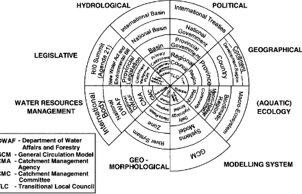
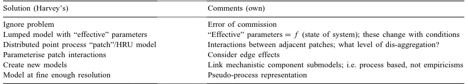
Fig. 1. Examples of vertical and horizontal scale interrelationships, taken from an integrated catchment management approach for the Kruger National Park, South Africa (after Jewitt and Görgens, 2000).
trade, or the paradigm shift in water resources from large-scale engineering works to smaller-scale envi-ronmental considerations, which have resulted in an appreciation that scaling is an important issue. Scal-ing, in fact, transcends all facets of organisational en-deavour in the natural (and other) sciences as well as in day-to-day governance. This is illustrated in Fig. 1 by some of the vertical and horizontal scale interre-lationships which have to be considered in integrated catchment management, in this example taken from the Kruger National Park Rivers Research Programme in South Africa (Jewitt and Görgens, 2000).
2. Objectives
associa-ted with scaling, nor the implications when interpret-ing their results. The objective of this paper is, there-fore, to highlight some selected conceptual as well as practical issues of scales and scaling in hydrology and agriculture by focusing on
• why scale and scaling problems arise;
• definitions and concepts of scale and scaling;
• key questions on, and some answers to, problems and methods of upscaling and downscaling;
• dis-aggregation to homogeneous landscape respon-se units (HLRUs) and the concept of re-aggregation;
• examples from the author’s researches of space/ time scaling issues from country to local scale in southern Africa;
• the types of errors associated with scaling; and
• some challenges perceived by the author in space/ time scaling applications of the “real world”. This is not a review paper on scaling in the con-ventional mode, for that has been done excellently in the past 5 years, particularly in the field of hydrology, through the many contributions making up recent special journal issues on scaling, for example, of the Journal of Hydrology, Water Resources Research, the Hydrological Sciences Journal, or Hydrologi-cal Processes, as well as through other publications by DeCoursey (1996), Harvey (1997) or Jewitt and Görgens (2000), the recurring contributions by Beven, Wood, Blöschl or Becker in the peer-reviewed literature, or in recent books edited by Feddes (1995), Kalma and Sivapalan (1995), Stewart et al. (1996) or Sposito (1998). Rather, this paper presents a perspective on certain foci when scales of space and time are transcended in the field of agrohydrology.
3. Methods
Numerous examples and case studies of scaling effects on agrohydrological responses in southern Africa make reference to the ACRU model. While a full model description is given in Schulze (1995), and in relation to updated model algorithms for climate change impacts in Schulze and Perks (2000), only a brief outline of relevant model features is presented below.
ACRU is a physical conceptual, daily time step model based upon a multi-level soil water budget
(Schulze, 1995). As a multi-purpose model, ACRU outputs daily values of runoff components (including stormflow, baseflow and peak discharge, which can be routed downstream through channels and dams), of reservoir status, sediment yield and irrigation supply/ demand as well as seasonal yields for selected crops grown either under rainfed or irrigated conditions. The model simulates evaporation from soil water and plant transpiration separately, thereby facilitating a CO2 physiological response option for modelling transpiration suppression in C3 and C4 plants with changes in atmospheric CO2 conditions. The maize yield algorithm includes a degree day driven phenolo-gical model, imbedded within the daily water bud-get, thus allowing for differential crop development and yield under varying temperature, rainfall as well as CO2 conditions. The model’s soil water budget components, runoff and sediment yield responses and crop yield simulations have been widely verified un-der a range of climatic and management conditions (e.g. Schulze, 1995; Kienzle et al., 1997).
The ACRU model has been linked by GIS to a southern African spatial and temporal database. In the context of this study, southern Africa consists of South Africa, Lesotho and Swaziland. This region of 1.293 million km2has been subdivided into 1946 so-called quaternary catchments (QCs), each being relatively homogeneous in its agrohydrological response (Schulze, 1997a; Schulze and Perks, 2000). Each QC has been assigned typical soil properties and also representative monthly means of daily maximum and minimum temperatures and monthly totals of potential evaporation (Schulze, 1997a), the last three attri-butes being converted within the ACRU model to daily values by Fourier analysis. The agrohydrol-ogy of each QC is driven by a 45-year (1950–1994) quality-controlled daily rainfall record which was de-rived from 1300 rainfall stations (Meier and Schulze, 1995).
4. Why do scale and scaling problems arise?
occur may be isolated. These are discussed below from the perspectives of hydrological responses and plant responses.
4.1. A perspective from hydrology
Six causes of scale problems with regard to hydro-logical responses may be identified (Harvey, 1997; Bugmann, 1997):
4.1.1. Spatial heterogeneity in surface processes Natural and anthropogenic landscapes display con-siderable heterogeneity (or patchiness) which influ-ence the types of processes which dominate and the rates at which they occur. These include the spatial and/or temporal variability of
• topography, e.g. altitude, aspect, slope, position in
the landscape (be it upland, midslope or footslope);
• soils, e.g. their infiltrability, transmissivity or water holding capacity, dependent inter alia on geology and topographic position;
• rainfall, e.g. its frequency of occurrence, persis-tence of wet or dry days, duration, intensity, sea-sonality or total amount;
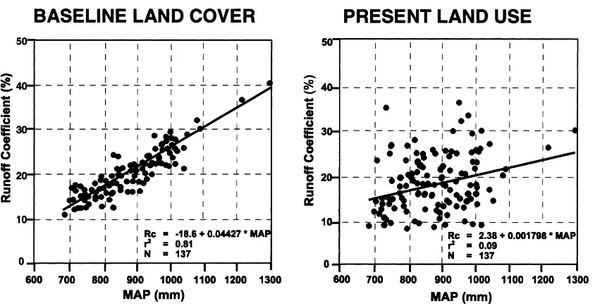
Fig. 2. Influences of land use on the rainfall:runoff relationship in the Mgeni Catchment, South Africa (after Kienzle et al., 1997; Schulze, 1998).
• evaporation, dependent on atmospheric demand (solar radiation, water vapour deficit and wind) in interplay with soil and vegetation characteristics;
• land use, accounting for factors such as the leaf area
index (LAI) and photosynthetic/stomatal characte-ristics of actively photosynthesising plants, canopy interception of rainfall, canopy height, structure and root distribution, as well as the degree of imper-viousness, and including effects of tillage practice and drainage.
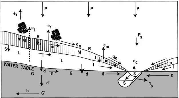
Fig. 3. Cross-section of a natural catchment system (after Moore, 1969).
runoff relationship has effectively been changed com-pletely by current commercial and subsistence agricul-tural, formal urban and informal peri-urban land uses (Kienzle et al., 1997; Schulze, 1998).
4.1.2. Non-linearity in responses
In Fig. 3, the cross-section of a catchment illustrates the various vertical (both up and down) and lateral fluxes which occur in the natural hydrological sys-tem. Clear distinctions in responses are made between hillslope processes (both on and below surface) and channel processes. Some processes occur episodically (e.g. rainfall), other cyclically (e.g. evaporation), still others ephemerally (e.g. lateral flows) or continually (e.g. groundwater movement). Another perspective is that certain responses are rapid (e.g. surface runoff), others at the time scales of days (e.g. lateral flows) or months (e.g. groundwater movement). These differ-ent rates of process responses introduce a high degree of non-linearity to the system, which is exacerbated when the natural system is replaced by anthropogenic systems such as land use changes or reservoirs.
4.1.3. Processes require threshold scales to occur Surface runoff generation, for example, involves two distinct processes each with a different threshold in order to occur. On the one hand, overland flow on high ground away from a channel is a process which occurs at a point in the landscape when rainfall inten-sity exceeds the infiltration capacity of the soil.
Satu-rated overland flow, on the other hand, is an areal process which requires a minimum upslope area over which lateral flows can accumulate and move downs-lope to saturate the area around the channel, with any rain then falling on the variably-sized saturated zone being converted to overland flow.
Subsurface flow generation, similarly, consists of two distinct thresholds. In this case, the threshold for interflow (i.e. subsurface lateral flow down a hillslope) to occur will depend, inter alia, on soil horizonation, different hydraulic conductivities along a hillslope toposequence (e.g. the crest or scarp or midslope or footslope) as well as on slope shape (e.g. concave, convex, uniform). On the other hand, the threshold for baseflow is determined by aquifer properties, the amount of recharge to groundwater that has taken place through either the soil profile or the channel and whether or not the groundwater level is “connected” or “disconnected” to the channel.
The threshold for the generated runoff to flow down a natural channel will be subjected to hydraulic laws which are determined, inter alia, by channel length, shape, roughness and slope. However, these thresh-olds would be modified markedly by human interven-tions through dam construction, canalisation or water transfers into or out of the system.
properties which, together with the occurrences and characteristics of localised small-scale storm events, would largely determine the shape of the hydrograph. On large catchments, on the other hand, the hydro-graph shape is often determined largely by hydraulic characteristics of channels and reservoirs as well as by occurrences and properties of large-scale regional rains of frontal and cyclonic origin.
4.1.5. Development of emerging properties
Emerging properties arise from the mutual inter-action of small-scale properties among themselves, for example, edge effects between landscape patches. These have different properties at large scale to the ones displayed by the same patches at small scale. A typical example would be the enhancement of evapo-ration at the edge of a well-irrigated field surrounded by a dry environment (the so-called “clothesline effect”), while over the irrigated field itself, if large enough, evaporation would be suppressed by a vapour blanket of air with a reduced vapour pressure deficit (the so-called “oasis effect”).
4.1.6. Disturbance regimes
Scaling problems immediately arise as a conse-quence of disturbance regimes being superimposed over a natural system, for example by the construc-tion of dams, draining of fields or changes in land use such as agricultural intensification or urbanisation.
4.2. A perspective from the plant
Plant systems are organised hierarchically, with many processes occurring across scales and many feedbacks taking place (Bugmann, 1997). Plants re-spond mainly via the photosynthetic process. Equally, therefore, as in the case of the hydrological system, scaling problems arise in plant responses especially with changes in atmospheric CO2 concentrations. Bugmann (1997) and Harvey (1997) have identified five causes of scaling problems in plant ecosystems.
4.2.1. Spatial heterogeneity combined with non-linearity
Plant systems may respond in a highly non-linear manner, particularly in multi-layered canopies, where there is vertical variation on leaf temperature, carbon fluxes, water vapour fluxes and light availability. In
natural ecosystems with a heterogeneous mix of com-peting plant communities, these non-linearities due to microclimate are often quite marked (Bugmann, 1997). Additionally, non-linearities may change under conditions of drought when compared to conditions of no plant water stress.
4.2.2. Feedbacks occur between plants and the surrounding environment
Under this scaling problem, Harvey (1997) gives two examples, both for conditions of enhanced at-mospheric CO2 levels. First, increased CO2 may lead to an increase in leaf area in the upper canopy. This would result in a decrease in light availability in lower canopies, and therefore, decreased leaf area there. Secondly, increased CO2 levels could reduce transpiration as a result of partial stomatal closure, resulting in reduced canopy humidity which, in turn, would lead to increased transpiration again!
4.2.3. Feedbacks and interactions occur between different plant components
For example, a change in atmospheric CO2 concen-trations would alter plant carbon to nitrogen ratios. This could result in a change in the allocation of C and N to roots and shoots which, in turn, would alter the photosynthetic response of leaves (Harvey, 1997).
4.2.4. Plants respond differently to changes in CO2 concentrations
The experimentally-determined differences in pho-tosynthetic responses to enhanced atmospheric CO2 concentrations between C3 and C4 plants are well documented in the climate change literature. Conse-quently, it is hypothesised that, in a future climate, the interactions among plant species will be altered. The implication is that no simple upscaling will be possible. This problem is exacerbated by the broader question of how plant communities acclimate to changes in CO2.
4.2.5. Disturbance regimes
Again, disturbance regimes, be they by hail occ-urrence, fire or sustained drought periods, will complicate scaling issues in plant systems, be they agricultural or natural.
pat-terns of, say, hydrological or plant systems at different scales. Relationships derived at one scale may not be applicable to another (cf. hillslope processes versus channel processes). The practical implication is that simplification in a model (e.g. by exclusion of certain processes and interactions) that is acceptable at one scale may not be applicable at another point. This is a point that needs to be borne in mind when modelling across a range of scales.
5. Scales and scaling: definitions and concepts
Scale may be defined as a characteristic dimension (or size), in either space or time or both, of
• an observation, or
• a process, or
• a model of that process
that encapsulates a usually discrete state of that pro-cess, or alternatively a transition between states of that process (Jewitt and Görgens, 2000). Intuitively, scale is an indication of an order of magnitude rather than a specific value.
Scaling, on the other hand, represents the tran-scending concepts that link processes at different levels in time and space (DeCoursey, 1996). One needs to distinguish between upscaling, i.e. the pro-cess of extrapolation from the site specific scale at which observations are made (e.g. rainfall at a mete-orological site) or at which theoretical relationships apply (e.g. the temporal redistribution of soil water according to Richards’ equation), to a coarser scale of study (e.g. the catchment or a GCM grid cell) and downscaling, i.e. taking output from a larger-scale observation or model (e.g. the synoptic weather situ-ation or a GCM grid cell) and deducing the changes that would occur at a finer resolution (e.g. in 1 h, or on a small catchment). Scaling, therefore, entails changes in processes, upwards or downwards, from a given scale of observation and thus includes the con-straints and feedbacks which may be associated with such changes. Included in the concept of scaling are changes in spatial and temporal variability, in patterns of distribution and in sensitivity. Scaling thus goes beyond simple aggregation (up) or dis-aggregation (down) of values at one level to achieve values at a more convenient level of consideration (DeCoursey, 1996).
Bugmann (1997), from an ecological perspective, distinguishes further between two different modes of upscaling. The first is implicit upscaling, in which scale-dependent features are taken into account while developing model equations, so as to formulate the model according to requirements of its particular site (e.g. accounting for the topographic effects of slope and aspect when modelling solar radiation receipt, or for tillage practices in crop yield). The second is explicit upscaling, i.e. using procedures that typically involve numerical simulations to scale up the response of the local model in space or time (e.g. assuming that the crop yield or hydrological response model developed and verified at field scale can be used for an entire country — this of course only holding true if there are no major scalar changes in the dominant pro-cesses such as local insect attacks or market-related forces in the case of crop production, or river abstrac-tions in the case of hydrological responses).
One needs to furthermore distinguish between types of scales and their characteristics as well as between the interactions between the types of scales. Concepts described below are taken largely from Blöschl and Sivapalan (1995) and from Jewitt and Görgens (2000). Process scales are defined as the scales at which natural phenomena occur. These scales are not fixed, but vary with the process. The intrinsic relationships between time and space scales are well illustrated by the so-called scope diagrams of which Fig. 4 is an example taken from processes relevant in hydrology.
The following features of process scales are impor-tant to note:
• Processes and their scales overlap; process scales are, therefore, relative rather than absolute in time and space.
• Events of small spatial scale are associated with short temporal scale (e.g. thunderstorms).
• Small-scale events display more variability than large-scale events (e.g. thunderstorms are usually highly localised and very rapid changes in rainfall intensity occur within them).
Furthermore, according to Blöschl and Sivapalan (1995), process scales possess three characteristics of both time and space. Temporally, one thus needs to distinguish
Fig. 4. Space and time interrelationships of processes relevant in hydrology (after Blöschl and Sivapalan, 1995).
• periodic processes, which have a cycle, or period (e.g. the rainy season, or evaporation being essen-tially a daytime process) and
• stochastic processes, i.e. probabilistic processes that
have a correlation length which is often expressed by the recurrence interval (e.g. a 1 in 10 year flood or drought occurrence).
Spatially, on the other hand, process scales exhibit
• spatial extent (e.g. the area over which the thunder-storm rainfall occurred);
• space period (e.g. the area over which a certain seasonality of rainfall occurs); and
• correlation space (e.g. the area over which the 1:10 year drought left its mark).
Observation scale is that scale at which humans choose to collect samples of observations and to study phenomena (Blöschl and Sivapalan, 1995). Observa-tion scales are determined by constraints of
• logistics (e.g. access to places of observation);
• technology (e.g. cost of state-of-the-art instrumen-tation); and
• perception (i.e. what is perceived to be important for a study at a given point in time).
• resolution, e.g. the density and distribution of a raingauge or experimental plot network within a country;
• grain, i.e. the coarseness of the sample (e.g. a
127 mm diameter raingauge, or a 22 m×2 m runoff plot or the level of accuracy in taking a sample), where a sample may be either coarse-grained (e.g. a catchment from which runoff is measured but the processes causing the runoff may not all be mea-sured and may thus be obscured) or fine-grained (e.g. an infiltration experiment in which all cause and effect is thought to be understood).
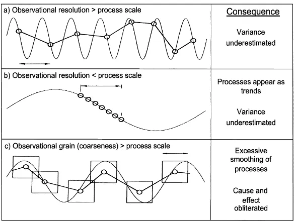
There is frequently a mismatch between the ob-servation and process scales. Ideally, obob-servations should be made at the scale at which the processes are taking place. Since, however, processes operate over a range of scales (cf. Fig. 4), this is seldom possible, in addition to there being logistical, technological and perceptual constraints. A problem arises when obser-vations are made at incorrect scales (e.g. in hydrology, with one rainfall and one streamflow gauge serving a catchment of 1000 km2, or in ecology where species mapping is often done at 1/4 latitude/longitude blocks) where one then has an idea of what is happening, but not why, or where within the study area.
Fig. 5. Observation vs. process scale relationships (after Blöschl and Sivapalan, 1995).
Furthermore, processes should ideally be observed over
• a large extent;
• with high resolution; and
• with fine grain
in order to allow any signal within the process to have been observed at the appropriate time scale. This is, however, rare, and thus, begs the question what the appropriate, or commensurate, scale is.
squares are visualised as an entire large catchment from which runoff is observed at a single outlet, the actual processes occurring within the large catchment have been excessively smoothed (one does not, for example, know where, within the catchment, it rained or soil was moist enough to generate the smoothly attenuated hydrograph) and the information has been largely aggregated.
The operational scale is the working scale at which management actions and operations focus. This is the scale at which information is available (e.g. in hydro-logical operations in South Africa at the scale of the QC, or population by census enumeration districts). Operational scales seldom concur with process scales because they are determined by administrative rather than by purely scientific considerations. They are thus not always scientifically meaningful, but may be con-venient and functional scales.
6. On up- and downscaling: some key questions
Both up- and downscaling procedures and assump-tions raise important quesassump-tions on scaling, some of which have also been highlighted elsewhere by Har-vey (1997) and Jewitt and Görgens (2000). Some key questions follow:
• When is simple aggregation (i.e. linear addition of elements) sufficiently accurate for upscaling? Band’s (1997) answer to this is that simple ag-gregation is possible only under uniformly wet or uniformly dry conditions over a large area or catch-ment, but that bias is introduced as soon as a spatial range of moist and dry exists within the catchment or during the wetting up or drying period or when lateral recharge is taking place.
• Are processes which are observed, or models for-mulated, at points or small spatial scales transfer-able to larger scales (e.g. can the lysimeter derived Penman–Monteith equation of potential evaporation be applied at the GCM grid cell level)?
• Where such scaling is possible, how should it be done?
• How do means change with scale?
• How does variability change with scale, where ability describes fluxes (e.g. rainfall) or state vari-ables (e.g. soil moisture) which vary over time and space?
• How does sensitivity change with scale, where sen-sitivity is a measure of the change in response of the dependent variable (e.g. crop yield) to a unit of change in a single driving or independent variable (e.g. rainfall), while holding all other variables con-stant? Under what circumstances would non-linear responses be either amplified or dampened as time scales become less frequent (e.g. in the 1 in 10 year event).
• How does heterogeneity change with scale, where heterogeneity describes properties which vary with space (e.g. a topographic roughness index, or prop-erties of soil)?
• How does predictability change with space, where predictability is the ease with which a system may be estimated? Certainly, at larger scales in catch-ment hydrology, the local heterogeneities of (say) variable topography, soils, land use or rainfall, each of which can dominate the hydrograph response over a small area, are averaged out and patterns appear more predictable.
• What type of conceptual errors are committed, wittingly or unwittingly, by scientists in their up-or downscaling assumptions?
• How can observations made at two scales be rec-onciled, for example by rescaling or application of fractals?
In this paper, some of these questions are answered or illustrated by way of example. In subsequent sections, issues of sensitivity and types of concep-tual errors are addressed more fully. An example of scaling and predictability follows below.
Fig. 6 illustrates relationships between predictabil-ity versus temporal and spatial scale. Predictabilpredictabil-ity,
according to Wiens (1989), is high when both the scales in time and space are similar. It would be low, however, when time scales are coarse but accompa-nying space scales are too fine. Similarly, when time scales are fine (e.g. 1 h) but the spatial scale is coarse (e.g. 300 km, as in the GCM output), an assumed high predictability resulting from the fine time scale being used is, in fact, a “pseudo-prediction” because of the time versus space scale mismatch.
7. On upscaling: towards solutions to the problem
The problem in upscaling, according to Wood and Lakshmi (1993), is that the macroscale model should preserve the statistical characterisation of the small scale variability (e.g. of topography, soils, or land use when considering more static variables; alternatively of sequences of wet/wet, wet/dry, dry/wet, dry/dry days or of extreme rainfall events when considering more dynamic variables), so that the macroscale can accurately represent the microscale fluxes associated with both event (e.g. rainfall) and inter-event periods (e.g. drying out or wetting up the soil profile).
In order to solve this upscaling problem, Harvey (1997) has proposed a sixfold hierarchy of possible solutions which are summarised in Table 1. Comments on these six “solutions” are from both Harvey (1997) and the author:
• The problem could be ignored. Assuming that an upscaling problem does not exist is, however, a grave “error of commission” — a term which is de-scribed later.
• A lumped model with so-called “effective” para-meters could be used. In lumped models, the area of interest (e.g. catchment) is considered to be a single entity, with variables (such as those representing
Table 1
A summary of possible solutions towards the upscaling problem (after Harvey, 1997)
Solution (Harvey’s) Comments (own)
Ignore problem Error of commission
Lumped model with “effective” parameters “Effective” parameters=f (state of system); these change with conditions Distributed point process “patch”/HRU model Interactions between adjacent patches; what level of dis-aggregation? Parameterise patch interactions Consider edge effects
Create new models Link mechanistic component submodels; i.e. process based, not empiricisms Model at fine enough resolution Pseudo-process representation
soils, land use or climate) being spatially averaged and model parameters being calibrated until the model output mimics observations “effectively”. However, such “effective” parameters are only representative of the state of the system (e.g. catch-ment) during the calibration period and should the state change, for example by land use or climate change, those calibrated parameters do no longer give “effective” results.
• The next level of refinement would be to use a distributed model in which processes observed at a point would be represented by a relatively homo-geneous “patch” or “hydrological response unit”. Questions which arise about such a distributed approach include the degree of “patchiness” or dis-aggregation from which to commence the up-scaling (see Section 9) and also the interactions between adjacent patches.
• A solution to the latter would be to parameterise interactions between patches, by considering edge effects such as advective processes.
• Creating a new model could be a next step towards solving the upscaling problem. This is, however, not a simple task because, to be more effective than previous solutions, a new model would have to link mechanistic and not merely empirical sub-models of the various components and should be based on phenomenological relationships, i.e. be process-based and not simply a logical sequential linkage of empirical relationships.
The problem of upscaling thus remains a largely unsolved one.
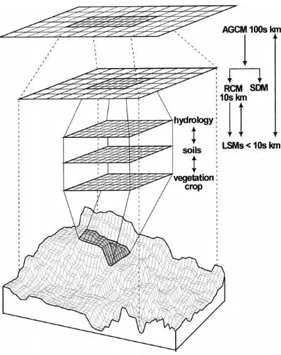
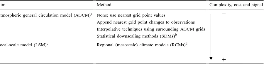
8. On downscaling: a brief discussion of methods and shortcomings
In downscaling, a dis-aggregation from a coarse to a finer scale takes place (Fig. 7) and in doing so the problem remains of parameterising the more detailed scale heterogeneity from the coarser spatial and tem-poral resolutions. More specifically, within the context of potential impacts of climate change, the major aim of downscaling is to facilitate the application of mod-els at the local scale (i.e.<10 s km) of actual catch-ments with their “real world” local water resources problems and on which actual crop yields may change, with consequences to actual farmers. However, such models would use atmospheric GCM input with spa-tial scale output at 100 s km intervals (Fig. 7). In this regard, Hostetler (1999) provides a hierarchy of down-scaling methods of increasing complexity and compu-tational effort/cost, but hopefully also with an increase in the signal of global to regional to local accuracy.
Fig. 7. Concepts of downscaling (after Hostetler, 1999).
Summarised in Table 2 , his methods are discussed below:
• The simplest “none”-method is merely to use the nearest GCM grid point values to represent the local scale. Essentially, no downscaling per se is applied and it is assumed (erroneously) that large-scale ef-fective parameters from the GCMs are adequate for the interpretation of impacts at finer scales.
• Nearest grid point changes to GCM output between, say, 2×CO2 and 1×CO2scenario runs, are ap-pended to present day values as anomalies. This method has the advantage of being very simple, with minimal computational requirements. The method maintains the intercorrelation structure of variables (e.g. diurnal and seasonal cycles), al-though the intercorrelation should also be viewed as a disadvantage (Hostetler, 1999).
• Regional bilinear interpolative techniques using values from surrounding GCM grid boxes may be applied. Such bilinear interpolation may either be simple or more complex, for example, when weighted by the inverse of the distance squared from the grid point. This remains a simple method, easy to use for gridded applications (e.g. Schulze and Perks, 2000), with the advantage that it main-tains regional structure by perturbing local climate patterns with the linearly interpolated indices of climate change. This method can thus be used, for example, to make temperature corrections for local elevation changes. It does, however, have the inher-ent disadvantage that certain primary GCM output parameters (e.g. pressure fields) may be unsuitable for direct use in intended impact models of hydro-logy and agriculture, and that large-scale secondary GCM output, e.g. precipitation fields are smoothed by the interpolative procedures to the extent that they may not display local dynamics which may control them (e.g. altitude).
• Statistical methods constitute one level up in down-scaling. Four sub-methods have been identified by Hostetler (1999), viz.
◦ linear and non-linear regression techniques;
rela-Table 2
Methods of downscaling from atmospheric general circulation models to local scales (after Hostetler, 1999)
Aim Method Complexity, cost and signal
Atmospheric general circulation model (AGCM)a None; use nearest grid point values
Append nearest grid point changes to observations Interpolative techniques using surrounding AGCM grids Statistical downscaling methods (SDMs)b
Local-scale model (LSM)c Regional (mesoscale) climate models (RCMs)d
aAGCM: atmospheric general circulation model. bSDM: statistical downscaling methods. cLSM: local-scale model.
dRCM: regional (mesoscale) climate model.
tionships are then applied to derive daily values of future precipitation and temperature values;
◦ stochastic weather generators: these use monthly climate change output to generate daily se-quences of precipitation and temperature which then account not only for changes in means but also for the possibly even more important changes in variability;
◦ use of probability distribution functions: despite being considered a relatively straightforward method of downscaling by Hostetler (1999), he stresses that these methods do make assumptions about underlying distributions and that one may question the assumption that stationarity will be maintained under conditions of climate change, particularly with regard to extremes of (say) precipitation and temperature, which are criti-cal processes in hydrologicriti-cal and agricultural responses, because one is inherently ascribing physical processes to statistical relationships.
• Regional mesoscale climate downscaling: this is a numerical technique using GCM outputs as initial and boundary conditions for regional-scale models. It is the most complex of the downscaling meth-ods described by Hostetler (1999). This method imbeds high resolution processes and feedbacks. It is amenable to interactive surface process mod-elling and can also be applicable to any type of climate change (i.e. intra- and inter-seasonal as well as decaded scale change), using fine resolution of both time and space. It is, however, a method which remains computationally demanding and time
con-suming, requires associated GCM simulations, is dependent on boundary conditions generated by the GCM and may, in fact, thereby introduce another level of model bias and error (Hostetler, 1999). Following on the above evaluation of downscaling methods, three points are identified which deserve fur-ther highlighting:
1. First, despite considerable recent scientific progress in statistical and regional mesoscale climate mod-elling, the standard downscaling technique used in country and continental studies of climate change impacts on hydrological and agricultural responses at this point in time (2000) remains interpolative techniques of one form or another, as described above.
any other intra-daily, inter-daily, or inter-seasonal variances.
3. Thirdly, the entire question around “transient/ invariate” controls and “superpositioning” in cli-mate change impacts studies remains an essen-tially unresolved downscaling issue. The concept of superpositioning revolves around transient cli-mate change occurring over a timespan of decades being superimposed over important invariate (i.e. non-changing) controls of the mesoscale climate such as altitude, physiography or continentality which influence local precipitation patterns (oro-graphic influences) or temperature patterns (e.g. lapse rates with altitude, or cold air drainage into valleys). These invariate controls and their signif-icance in agrohydrological responses will persist, irrespective of any larger synoptic shift associ-ated with climate change, but their profound local influences will have to be separated out for in-dividual synoptic conditions from more regional perturbations (Schulze, 1997b).
9. On dis-aggregation to homogeneous landscape response units
In order to obtain HLRUs for use with models to upscale responses of the hydrological and agricultural systems, the typical approach would be to overlay GIS coverages of attributes such as soil, geology, topo-graphic characteristics, climate parameters and land use, where each attribute is subject to a classifica-tion system, to produce a mosaic of separately delin-eated natural landscape elements, each of which may be considered internally homogeneous and is assumed to behave uniquely. Similarly classified units, which may be repeated in the patchwork landscape, are as-sumed to behave identically. These joint occurrences of fundamental elements making up the HLRUs go by many other names in the literature, for example, func-tional response units (FRUs), aggregated simulation areas (ASAs), hydrological response units (HRUs) or hydrotopes (Becker and Braun, 1999). HLRUs can be represented either as vectors (irregular polygons) or as rasters (grid boxes, pixels).
The challenge to modellers is to assign effective parameter values to different HLRUs, and this presents numerous problems of scaling.
9.1. Scaling processes
In the delimitation of HLRUs, cognisance has to be given to three scaling processes, viz.
• vertically identified scale processes, e.g. distribution of soils or land use which may be distinguished from maps or GIS images;
• horizontal scale processes, e.g. atmospheric pro-cesses such as direction of rain bearing airmasses, wind or advective processes — usually an ignored scale issue; as well as
• lateral-scale processes, e.g. different slopes and aspects intercepting different solar radiation load-ings which result in different potential evaporation demands, or unequal redistribution of soil water as a consequence of position along a hillslope’s toposequence — again, a frequently ignored scale consideration (discussed in more detail under Section 9.4).
9.2. Classification
The type and detail of the classification system can be critical with regard to the similarity of behaviour of an HLRU:
• For example, land use type may be classified in the GIS coverage according to planning criteria, where such a classification is not all that useful in terms of hydrological response behaviour. Similarly, soil type can be classified pedologically rather than hy-drologically. In both examples, the classification would, if hydrological modelling were to be un-dertaken, have to be “translated” into hydrological variables (Schulze, 1995).
Fig. 8. Schematic of lateral flow representation in the ACRU model.
9.3. Compatible process representation
In considering the scale detail of HLRUs, a for-gotten question is often as to which process domi-nates the response. HLRUs may represent soil/land use/topography differences very well, but often the dominant spatial forcing function of response is rain-fall distribution, particularly if it is convective in na-ture. If the rainfall representation is poor (e.g. sparse network of raingauges) and the spatially defined at-tributes are very detailed (e.g. of land use and soils), then a scaling “break down” may occur because the detailed HLRUs, in fact, represent pseudo-detail not matched by the detail of rainfall information. Ide-ally, the scale representation of all attributes used in delimiting HLRUs should have similar sensitivity.
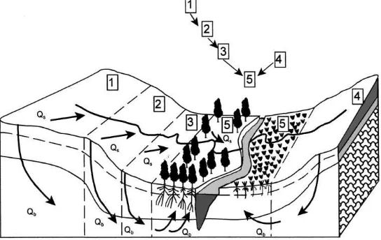
9.4. Lateral processes
The realisation of the importance of subsurface flows, and of the unequal distribution of soil water across a hillslope transect from crest through scarp to midslope and footslope to the riparian floodplain zone, as well as the variable source area concept of runoff generation have come to the fore in recent years. This realisation takes on even greater signifi-cance now that the movement of natural and artificial pollutants is becoming an environmental issue and the role of the riparian zone in catchment manage-ment is beginning to be addressed. The significance
of lateral-scale processes in catchment management is illustrated in the example below. Fig. 8 shows schematically how stormflows (Qs) and baseflows (Qb) of the different slope segments (1–5) are rep-resented in the ACRU model (Schulze, 1995) when a catchment’s delineation into HLRUs takes account of lateral slope segments. In a simulation which as-sumed that the four slope segments to the left of the stream were of equal area, and then planting up the riparian zone (5) with deep rooted evergreen Euca-lyptus grandis trees, while the other three segments (1–3) had shallow rooted grassland (veld) at Cedera in South Africa (29◦34′S, 30◦14′E, MAP 870 mm,
altitude 1205 m) gave a mean annual runoff (MAR) 15% lower (126 versus 149 mm) and a coefficient of variation of annual flows 9% higher (112 versus 103%) than when the same area of trees was planted on the crest (segment 1) and the riparian zone was replaced with shallow rooted grassveld.
10. From dis-aggregation to re-aggregation
explain both the signal and the variances of the re-sponse. If the dis-aggregation is too coarse, one has to assume that the “dominance” principle applies, viz. that each HLRU responds similarly to that of the dom-inant land use or soil within it, in which case many of the variances resulting from interacting non-linear responses of important, but non-dominant, processes cannot be explained.
At the other end of the scale, the dis-aggregation may become so detailed that there can be dis-aggrega-tion “overkill”, primarily because of the ease with which HLRUs can nowadays be created from GIS overlays by using just a few commands. Scientists may then become intrigued by detail rather than by the actual scaling problem they are trying to resolve. With the resultant multitude of disconnected HLRUs they may have created, a number of pertinent ques-tions arise:
• Are the many HLRUs identified actually all res-ponding differently (which is, after all, the purpose of dis-aggregation) or do many of them display sim-ilar behaviour?
• Does the high degree of dis-aggregation actually improve simulation results, or is a point reached in dis-aggregation at which goodness-of-fit statistics between simulated and observed no longer improve and, in fact, may be regressing?
• Is noise beyond signal eventually being created with further dis-aggregation?
This leads to the concept of re-aggregation, whereby a re-lumping of equi-response units is un-dertaken, with due consideration given to lateral and subsurface processes occurring in a landscape, into what have been termed “hydrotopes” in an hydrolo-gical context (Becker, 1995; Becker and Braun, 1999). The procedure adopted in Becker and Braun (1999) is an excellent example of hydrological re-aggregation, viz. to apply a sensitivity analysis between simulated and observed values according to pre-selected fit-ting criteria (e.g. r2, coefficient of efficiency). They then combine HLRUs which are similar in behaviour until the goodness-of-fit criteria either drop below a predetermined limit, or any further re-aggregation displays a natural break in goodness-of-fit. What has to be borne in mind when re-aggregating is that one should distinguish, when combining HLRUs, between elements of the natural landscape (e.g. to-pography, wetlands, climate, soils) and the “human”
landscape (e.g. land use and land management practices).
A question frequently posed is whether there is a preferred scale at which to model. Considerable theo-retical work has been undertaken in scaling theory, resulting in concepts such as the representative ele-mentary area or applications of fractals or rescaling. These concepts are important in improving our un-derstanding of scaling, and such scientific approaches may be applicable in a relatively unperturbed natural landscape. However, most real landscapes in which scaling issues occur are human-modified landscapes in which theoretical scaling concepts are not always any longer valid, in hydrology for example because of river abstractions, return flows, construction of dams or canalisation, all of which alter considerably the nat-ural flow regimes, and hence, scaling laws.
The question of dis-aggregation and preferred scale in real world situations thus often becomes a problem-determined one which changes from case to case.
11. Space and time scaling: examples from southern Africa
Following on the discussions on types of scale and up- and downscaling, examples of the application of scaling issues are presented from a southern African perspective, at both country level and local level.
11.1. Mesoscale representation of a country-level sensitivity analysis of hydrological responses to climate change forcing over southern Africa
Sensitivity analysis can be undertaken to establish the extent to which a driving variable in a system is sensitive to change, in which direction the sensitivity tends and whether the sensitivity is spatially uniform or heterogeneous. Such analysis is particularly impor-tant where uncertainty exists as to the importance of change to that variable in a system.
Climate change can impact runoff generation by changes to three variables:
actively photosynthesising biomass (LAI) and soil water availability. Hydrologically, the hypothesis is that through (say) a doubling of CO2levels, transpi-ration would be reduced, the soil profile would thus be relatively moister and runoff would increase.
• Increases in temperature result in a higher atmo-spheric demand, and hence, potential evaporation. Hydrologically, it is then hypothesised that soil water evaporation between rainfall events would increase, as would transpiration demand, with the relative importance of the two processes dependent on biomass cover. The resultant drier soil should thus generate less runoff, conditional upon precip-itation and CO2levels being held constant.
• Any changes in precipitation would change both antecedent soil moisture conditions and the indi-vidual event’s magnitude, thereby changing the runoff response.
To assess the respective mesoscale spatial sensitivi-ties of these three forcing variables, the ACRU model was run for a 45-year daily rainfall record on each of the 1946 QCs covering southern Africa, in each case changing a single variable at a time while holding the other two constant at present values (Schulze and Perks, 2000). Fig. 9 (top) shows that transpiration sup-pression in a 2×CO2atmosphere is, by itself, hydro-logically relatively insensitive according to the ACRU model, with MAR generally increasing by only 2%, except in wetter regions with longer periods of active plant growth, where it can increase the MAR by up to 8%. A 2◦C temperature increase, on the other hand,
reduces MAR by <5% to 0.95 of the present runoff over most regions (Fig. 9, middle). However, in cooler high-altitude areas and particularly in the winter rainfall regions of the southwest, an increase in tem-perature by itself can become a critical variable in the impact of climate change, with the enhanced evap-otranspiration changing soil moisture regimes to the extent that MAR could be reduced by up to 50% in places. Runoff responses in southern Africa remain most sensitive by far to changes in precipitation, how-ever, with a unit1P (e.g. by 10%) generally resulting in a two to four times unit change in runoff (i.e. 20–40%). This response increases to five times in the winter rainfall regions where antecedent soil moisture conditions remain wet in the inter-rainfall event pe-riods because of low winter-time evapotranspiration (Fig. 9, bottom).
This analysis shows clearly the considerable spa-tial differences in sensitivity which can exist in a complex, interactive hydrological system, and hence, stresses the value of such analyses being undertaken at mesoscale level.
11.2. Mesoscale representation of a country-level sensitivity study of maize yield change to the CO2 fertilisation effect with climate change over southern Africa
A great deal of uncertainty exists as to whether the laboratory-determined CO2 “fertilisation effect” influences on plant growth through changes in photo-synthetic responses and water use efficiency (partially by the transpiration suppression described above) will actually manifest themselves under large field con-ditions. Equally, uncertainty, therefore, exists as to whether the algorithms imbedded in agrohydrological models such as ACRU represent this “fertilisation effect” realistically. To assess the mesoscale sensi-tivity of this uncertainty, the differences in QC level maize yields between a “future” and present climate were assessed with the CO2 feedback switched on versus switched off, using the ACRU maize yield module (Schulze, 1995) with a plant date of 1 Novem-ber (Fig. 10). For the “future” climate, the region-alised monthly changes in maximum and minimum temperatures as well as precipitation for a 2×CO2 scenario from the 1998 version of the Hadley GCM (excluding sulphate feedbacks) was used to perturb the 45-year present day daily rainfall and temperature series for each QC with MAP>300 mm.
The significant mesoscale regional differences be-tween changes in maize yield when just one uncertain feedback variable is either switched on or off (Fig. 10) highlights again the value of sensitivity analysis in space/time scale studies.
11.3. Inverting the time scale in a country-level threshold analysis of critical change in runoff with climate change, mapped at mesoscale
CO2conditions in, say, 60 years from the present. In such impact studies, the time scale is fixed, but the response varies spatially. What conventional analyses, therefore, identify is where, say 60 years from now, the specific response may be more significant than else-where. However, those studies do not indicate when (over the next 60 years) a critical threshold level of change is likely to occur at different locations within a study region.
Such threshold analyses may be undertaken by ef-fectively “inverting” the timescale. Assuming that a 10% change (+or−) in MAR was a critical threshold of change, Fig. 11 illustrates, for the 1998 version of the Hadley GCM output, where such a 10% change is likely to occur with over time, e.g. by the year 2015, 2030, 2045 or only by 2060. Details of the technique are given in Schulze and Perks (2000). Such an inver-sion of the time scale of a likely climate change im-pact implies that water resources planners could take
Fig. 11. Threshold analysis of assumed critical runoff change with climate change over southern Africa (after Schulze and Perks, 2000). necessary adaptive measures earlier in certain critical regions than in others.
11.4. Downscaling seasonal rainfall forecasts to daily values for country-level modelling of seasonal runoff forecasts
As an alternative to assessing climate change pacts over decadal time scales, climate variability im-pacts may be more useful in more immediate decision making at inter-annual time scales. An example of this follows.
be correct one third of times, and any forecast correct more than 33% would have “skill” to it. In climates with a high inter-seasonal variability of rainfall, it is hypothesised that, if rainfall season forecasts are of sufficient skill, that they would be “translatable” into seasonal forecasts of crop yields or streamflows by ap-propriate models for critical food security or water re-sources decisions to made. Simple downscaling tech-niques were used in a recent initial study of seasonal streamflow forecastability in South Africa (Schulze et al., 1998).
The summer rainfall zone of South Africa has been classified into six forecast regions. All QCs falling within a specific forecast region were assumed to have the same seasonal categorical rainfall forecast. Historical forecasts of rainfall categories A, N or B for the main rainy period December–March were ob-tained from the Climatology Research Group of the University of the Witwatersrand for the 15 seasons 1981–1982 to 1995–1996 (Table 3). When compared with the observed December–March rainfall cate-gories for those years, the forecast skill was found to be 50%, with some regions’ seasonal rainfalls be-ing more forecastable than those of others, and some years forecast better than others (1981, 1987 and 1990 forecasts were incorrect in all six regions, while 1982 and 1991 were correct in all six regions; Table 3).
In order to undertake an initial evaluation of sea-sonal runoff forecastability, the categorical seasea-sonal rainfall forecast first had to be downscaled to daily values for use in the ACRU model. This was achieved in each QC by taking its 45-year daily accumulated observed rainfall record for the December–March pe-riod and categorising years as A, N or B according to their ranking in the top 15, middle 15 or lower 15 of the 45 years (Schulze et al., 1998). If a forecast was (say) A, i.e. in the above-normal rainfall category, than a representative year’s observed December–March rainfall from the A-ranked years was extracted. For a given year, a runoff simulation with ACRU was then run with observed daily rainfall data until 30 Novem-ber, and thereafter with the extracted representative year’s daily rainfall for the forecast category. The simple hypothesis was that, if the seasonal runoff from the forecast rainfall (downscaled to daily values) was closer to the seasonal runoff from observed daily rainfall than the long-term median seasonal runoff, then a hydrological benefit (“win” situation in Fig. 12)
would have been derived from using the categorical rainfall forecast; if not, then no benefit was derived (“lose” situation in Fig. 12) and if the seasonal runoff differences were within 5%, the rainfall forecast was assumed to have made no difference.
Fig. 12 shows that the application of the above simple temporal downscaling techniques, particularly under conditions when the seasonal rainfall skill may be considered to be reasonably accurate (e.g. when totally incorrect forecasts for years 1981, 1987, 1990 are removed), can be potentially beneficial for sea-sonal runoff forecasts and that such information is thus potentially useful to water resources operators. Similar scaling methodologies could be used to assess the benefits of crop yield forecasts.
11.5. Spatial scaling in mountainous terrain: the case of crop yield variations with altitude, aspect and gradient
Mountainous terrain at hillslope and valley levels present special challenges to spatial scaling for, in ad-dition to having to contend with more conventional downscaling procedures, the local climate assumes more complex dimensions through influences of alti-tude, aspect and slope gradient.
Solar radiation loadings in mountainous terrain, for example, can vary markedly at different altitudes, slopes and aspects as a function of latitude, time of year, time of day, atmospheric conditions of turbidity, degree and type of cloud, topographic shading from surrounding hills and re-radiation from surrounding hills. Numerous models exist to quantify these ef-fects on solar radiation, and one which can account for all the factors listed above is the Radslope model (Schulze and Lambson, 1986). Solar radiation, in turn, is a major forcing variable of temperature as well as radiation-driven potential evaporation equations such as that by Penman (1948), which can also be simu-lated on sloping terrain with the Radslope model. In addition, temperature lapse rates with altitude vary in mountainous terrain by region, season and tempera-ture parameter (Schulze, 1997a). Solar radiation, tem-perature and potential evaporation are all important input variables in more crop-detailed yield models.
Fig. 12. Simple benefit analysis of applying downscaled seasonal categorical rainfall forecasts to forecasts of runoff in South Africa (after Schulze et al., 1998).
South Africa (29◦05′S, 29◦27′E) at altitudes ranging
from 1000 to 3000 m, together with locally obtained daily rainfall, the influence of mountainous terrain on maize yield (Zea mais) was simulated using the CERES 3.0 maize yield model (Jones et al., 1998). Model runs were performed at three altitudes, viz. 1000, 2000 and 3000 m, in each case for a warm aspect (i.e. north facing in the southern hemisphere) and a cool aspect at respective slope gradients of 0, 10 and 30◦. From Fig. 13 (top), it may be seen how
simulated maize yield varies under present climate conditions from zero yield at high altitude (where temperature and/or solar radiation thresholds are too low for plant physiological requirements to be met) to 8.4 t/ha at hotter, lower altitudes. For the climate change scenario which is indicated in Fig. 13 (bot-tom), it is significant to note that, at the lower al-titudes, there is a yield reduction (temperatures too high), while at 2000 m, where present temperatures
are too low for high yields, yields may increase by over 6 t/ha, particularly on warm aspects.
This case study has illustrated clearly how differ-ent spatial scale considerations become important in mountainous terrain under present, but particularly under possible future climates, when new thresh-olds for response not reached under present climatic conditions may be met. It is for this reason that mountainous regions are highly sensitive to climate change and deserve special attention at the appropriate scale.
12. Types of errors associated with scale issues
all the various scaling errors which they may incur. Haufler et al. (1997) has identified two types of scale errors which occur frequently and this twofold classi-fication has also been elaborated upon by Jewitt and Görgens (2000).
12.1. Errors of omission
Defined by Haufler et al. (1997) as errors which occur “when a model fails to predict the occurrence of a process that is actually present in an area”, the following examples illustrate the concept of errors of omission:
• Relevant questions are not asked in the model because they are not obvious at the scale being considered, for example, when a crop yield model fails to take cognisance of hail, pests or diseases; alternatively, when a daily hydrological model fails to consider effects of rainfall intensity, duration or timing in the course of the day.
• Focus on a single scale may obscure important processes that only become obvious at either finer or broader scales, for example, applying projected mean monthly changes in temperature and rainfall from a GCM to perturb present daily time sequences in climate change impact studies with no indication of future changes in day-to-day persistencies of wet/dry days or changes in daily extreme values.
• They may fail to ask questions about cumulative impacts on a broader scale than that being studied, for example, failure to appreciate possible cumu-lative impacts of over-irrigation, and resultant per-colation of fertilisers into the groundwater system, on eutrophication of dams downstream.
• They may fail to examine large-scale impacts on a smaller scale, for example, failure to model the effect of anthropogenically induced temperature change on different slopes and aspects at local scale.
12.2. Errors of commission
This second type of error, defined by Haufler et al. (1997) where “the occurrence of a process is erro-neously predicted in an area where it is not present”, is tantamount to acknowledging that one is wrong in a scalar assumption, but is nevertheless committed in
the model to continuing with that error of scaling. Two examples follow:
• Questions may be asked at a scale at which meaningful answers cannot be provided, or what Meentemeyer (1989) has termed “calculating the outcome of macrolevel (aggregate) relationships based on microlevel (individual) relationships”. Examples include the assumption that the lysime-ter derived Penman–Monteith evapotranspiration or laboratory-derived Green–Ampt infiltration equations can be applied at global scale. These equations, may, in fact, give realistic results be-cause they are bounded by upper and lower physical conditions. These are nevertheless scale “transgressions” which are often made, possibly because the small-scale equations may appear mathematically elegant, but in full knowledge that simple spatial upscaling is a misrepresentation of the original intent of the equation.
• The assumption may be made that the appropriate scale for a given process is the same for all compo-nent processes of the system, e.g. when upscaling the streamflow process assuming that the stormflow generation, interflow and baseflow components can all be upscaled identically with no consider-ation given to the individual spatial and temporal dynamics of each component.
13. Discussion and conclusions
Scaling challenges which face hydrologists and agriculturists relate to both top–down and bottom–up research. Some challenges identified by this author are elaborated upon below.
13.1. Top–down research
• In top–down research the effective spatial and tem-poral downscaling from GCMs to operational land-scape units at which climate and climate change impacts really matter to the population at large remains a core problem. This is particularly so in systems where precipitation is a sensitive forcing variable, as in hydrology and agriculture, and to this day it remains a scaling mismatch that the abil-ity of GCMs to predict spatial and temporal change in precipitation declines from global to regional to local scales while the importance of precipitation in agrohydrology increases from global to regional to local scales, particularly in semi-arid countries (Schulze, 1997b).
• Another core top–down problem identified in spa-tial downscaling remains that of superpositioning, i.e. the local interactions between synoptic-scale climate systems being superposed onto invariate local physiographic controls of rainfall and tem-perature and how these local controls may change in future.
• In regard to temporal downscaling the “mean ver-sus variability” scaling paradox is as yet largely unresolved, viz. that GCMs at present give broad indications only of directions and magnitudes of means of changes in precipitation and temperature, while impact studies require detailed information on their variability, with timescales at intra-daily, inter-daily and inter-seasonal levels, as well as in-formation on persistencies of events (e.g. sequences of hot/hot, hot/dry, etc. days or wet/wet, wet/dry etc. days).
• Further on the top–down research agenda is the problem of estimating daily point and spatial rain-fall distributions (magnitudes, persistencies) in an era of declining conventional climate observation networks. This introduces scaling errors in space (sparse networks) and time (short records). Reli-able and readily availReli-able (especially to developing countries) daily rainfall values are eagerly awaited
from remote sensed sources transmitted by satellite or from ground-based radar.
13.2. Bottom–up research
One bottom–up research challenge is the appropri-ate upscaling of processes observed at small scale for use at meso- or GCM scale. The direct applications of the Penman–Monteith estimation of evapotranspi-ration or the Green–Ampt equation for infiltevapotranspi-ration over large areas remain serious “errors of commission” in climate change despite the fact that they appear to yield realistic results. Two further bottom–up scaling research needs are identified, both dealing with im-pacts models in agrohydrology:
• The first of these is for the models to display com-patibility between the various process representa-tions making them up and not have some processes represented in great detail while others are presented as oversimplifications.
• The second is that the impact models frequently do not cope with extreme temporal-scale events (such as heat waves, fire, soil profile saturation or hail) in the way natural systems do, and this problem requires to attention of model developers.
13.3. Addressing scale issues of the “real world”
Final concluding thoughts revolve around address-ing what, in the perception of this author, may be called scale issues of the “real world”, commencing with those related to temporal scales.
• For “real world” decision making particularly in the developing world, a plea is made to re-focus on daily time step modelling. Diurnality is a natu-ral time scale. Diurnality furthermore encapsulates important agrohydrological processes, persistencies and episodic events. Many operational decisions in agriculture and hydrology are made according to daily atmospheric conditions or soil moisture states, e.g. tillage, harvesting, or irrigation. Furthermore, historical daily climate data are available in much greater abundance (by network density and length of record) than that of shorter steps, facilitating risk analyses to be undertaken with some confidence.
sea-sonal climate forecasts (as against decadal time scale research). Especially in areas where telecon-nective signals with, say, sea surface temperatures or the Southern Oscillation Index are strong, sea-sonal climate forecasts can be of great immediate benefit to society, especially in semi-arid or lesser developed regions, when “translated” into food or water security attributes which can be used in operational decisions. This is particularly the case with seasonal forecasting skills now improving and their benefit:cost ratios increasing.
With regard to “real world” issues and spatial scales, three scales are identified by this author at which fur-ther research would be beneficial:
• The first is at the hillslope scale, for it is at this scale that certain runoff generating mechanisms can play a dominant or less dominant role, and we need to understand these better in order to model important biogeochemical and riparian zone processes with more confidence.
• The second is the field-to-farm scale, for this is a discrete operational unit in agriculture at which many decisions are made and at which data are col-lected, be it at subsistence or commercial farm level.
• The third scale is that of the operational catch-ment, the non-gridded, non-experimental catchment at which real decisions on water storages, releases, return flow and quality are made, and for which short or long-term hydrological forecasting is an im-portant consideration. This operational catchment is likely to be small in developing countries and larger in developed countries.
Finally, the complexities of issues of scale and scaling in the natural environments in which agri-cultural and hydrological systems operate cannot be overstressed. Unfortunately these scale issues are often exacerbated by anthropogenic actions (e.g. tillage or drainage in agriculture; construction of reservoirs and canals in hydrology), for our man-agement actions within these systems inevitably interrupt natural scaling processes, thereby com-plicating matters further. As natural scientists we should consciously remind ourselves of issues of scale, for unwittingly rather then purposely we of-ten do not give enough consideration to the tran-scending and interactive characteristics of scales and their consequences in our scientific endeavours and interpretations.
Acknowledgements
This paper was first presented at the GCTE Focus 3 Conference on “Food and Forestry: Global Change and Global Challenges” in Reading, UK in September 1999. It was prepared while the author was on sabbat-ical leave from the University of Natal at the Institute of Hydrology in Wallingford, UK. The Institute, the National Research Foundation of South Africa and Elsevier Science are thanked for their support of this project. Some the results from case studies emanate from research supported by the Water Research Com-mission and the South African Country Studies for Climate Change Programme. Those institutions as well as colleagues L.A. Perks, M.J.C. Horan, G.P.W. Jewitt and G.A. Kiker are thanked for their various contributions to this paper.
References
Acocks, J.P.H., 1988. Veld Types of South Africa. Botanical Survey of South Africa, Memoirs, Vol. 57. Botanical Research Institute, Pretoria, p. 146.
Band, L.E., 1997. Ecosystem processes at the watershed scale: scaling from stand to region. In: Hassol, S.J., Katzenberger, J. (Eds.), Elements of Change 1997 — Session One: Scaling from Site-Specific Observations to Global Model Grids. Aspen Global Change Institute, Aspen, CO, USA, pp. 40–46. Becker, A., 1995. Problems and progress in macroscale hydrologic
modelling. In: Feddes, R.A. (Ed.), Space and Time Scale Variability and Interdependencies in Hydrological Processes. CUP, Cambridge, p. 135.
Becker, A., Braun, P., 1999. Disaggregation, aggregation and spatial scaling in hydrological modelling. J. Hydrol. 217, 239– 252.
Beven, K.J., Fisher, J., 1996. Remote sensing and scaling in hydrology. In: Stewart, J.B., Engman, E.T., Feddes, R.A., Kerr, Y. (Eds.), Scaling up Hydrology Using Remote Sensing. Wiley, Chichester, UK, pp. 1–18.
Blöschl, G., Sivapalan, M., 1995. Scale issues in hydrological modelling: a review. Hydrol. Processes 9, 251–290.
Bugmann, H., 1997. Scaling issues in forest succession modelling. In: Hassol, S.J., Katzenberger, J. (Eds.), Elements of Change 1997 — Session One: Scaling from Site-Specific Observations to Global Model Grids. Aspen Global Change Institute, Aspen, CO, USA, pp. 47–57.