An Efficient Procedure For Activating Bi-State Actuator Arrays Using Neuro-Fuzzy Network

Subject: IES 2012: Paper Notification

From: Admin IES 2012 (ies@eepis-its.edu)

To:

felixpasila@yahoo.com;

Date: Friday, August 3, 2012 10:22 AM

Dear Felix Pasila,

We are pleased to announce that your paper is ACCEPTED in IES 2012. The evaluation of your paper and

all comments from reviewers of your paper are enclosed to this message. We hope that you can take them

into account as much as possible in preparing the camera ready of your paper in order to accomplish a high

quality paper.

Title : An Efficient Procedure For Activating Bi-State Actuator Arrays Using Neuro-Fuzzy Network

Author : Felix Pasila,,,,,

Status : ACCEPTED

And the aspects bellow is the scale of assigning score :

6 : Strong Accept (Excelent quality, cutting-edge ideas)

5 : Accept (Good quality, sound and interesting results)

4 : Weak Accept (Vote acceptance, but won't argue for it)

3 : Weak Reject (Don't like it, but won't argue against it)

2 : Reject (I will argue to reject this paper)

1 : Strong Reject (Unsuitable for publication in this forum)

---

================================================

Reviewer 1

Relevance Aspect : 5

Originality Aspect : 5

Significance Aspect : 5

Technical Aspect : 4

Clarity Aspect : 4

Overall Aspect : 5

Positive Aspect : hasil eksperimen menunjukkan efektifitas metode yang digunakan

Negative Aspect : aktuator hanya digunakan dalam 2 dimensi

Additional Comment :

---

================================================

Reviewer 2

Negative Aspect :

Additional Comment :

---

We would like to inform you that the deadline of Final Manuscript Submission (camera ready) is on August

16, 2012.

We also would like to inform you later about the registration process. We are looking forward to seeing you

at the conference in IES 2012, Surabaya,Indonesia.

Sincerely Yours,

Amang Sudarsono

IES 2012 General Chair

Subject: Re: Internet Banking Mandiri - Fund Transfer: IES 2012 for Felix Pasila

From: Zaqiatud Darojah (zaqiah@eepis-its.edu)

To:

felixpasila@yahoo.com;

Date: Thursday, October 11, 2012 10:36 AM

Yth. Bapak Felix Pasila

Salam hormat,

Terimkasih atas konfirmasi dan partispasinya pada Seminar IES 2012 Bapak Felix. Kami tunggu kehadiran

Bapak pada pelaksanaan IES tanggal 24 Oktober 2012 di Politeknik Elektronika Negeri Surabaya. Atas

perhatian dan kerjasama Bapak, kami mengucapkan terimakasih.

Hormat kami

Panitia IES 2012

---

EEPIS - Bridge To The Future

An Efficient Procedure For Activating Bi-State

Actuator Arrays Using Neuro-Fuzzy Network

Felix Pasila

Electrical Engineering Department Petra Christian University

Surabaya, Indonesia felix@petra.ac.id

Abstract— A novel approximation procedure based on hybrid neuro-fuzzy (NF), called Takagi-Sugeno real-input multi-binary-output (TS-MIMO) neuro-fuzzy network, is proposed to control the bi-state actuator arrays. This efficient procedure is used in static force mechanism of 2D-rigid body manipulator. The proposed NF model employed off-line neuro-mechanism using Levenberg-Marquardt algorithm (LMA) and Takagi-Sugeno model as inference system in fuzzy systems. Additional hill climbing method as optimal searched procedure improved the minimum error in the learning computation. Simulation results are provided not only to demonstrate the efficiency of the NF model in activating the bi-state in arrays, but also to explain how to find the minimum number of actuators that should be put in the rigid body system. These first results will lead the NF mechanism as a universal force control for bi-state actuator arrays.

Keywords: NF type TS-MIMO procedure, general approximator, bi-state actuator arrays, one-DOF manipulator, force control fashion

I. INTRODUCTION

Binary manipulators have been used in several applications and played significant roles, especially in robotics and biomechanics applications [1,2,3,13]. These bi-state manipulators are particular kind of discrete device, in which the states flip between two possible values, such as activated-not activated, open-closed or contracted-relaxed (e.g. pneumatics, dielectric elastomer actuators, shape memory alloy). Because of the states condition, binary manipulators have several potential benefits compared to continuous manipulator systems, for example: they are relatively inexpensive and lightweight; minimal support devices because they can be operated without extensive feedback control. In contrast with the advantages, they have problem in actuating the binary states, especially when the manipulators have a massive number of actuators.

Concerning the control strategy, some previous works has been done related to discrete-actuated manipulators control. For instance, from the mid 1990s, Chirikjian [1,4] proposed a variety of efficient algorithms for trajectory tracking approximation of binary manipulators. In these algorithms, the manipulators are actuated by binary actuators that placed in a serial-parallel configuration with position control approach. They also introduced the new concept of discretely actuated manipulators called an extended Ebert-Uphoff algorithm [2,3],

which considering the full position-orientation of inverse kinematics problem rather than the pure position problem. This algorithm gives many influences to researchers, such as constructing hyper-redundant manipulators based on mathematical model and controlling the desired position-orientation of end-effector.

In contrast with position control fashion, not many researchers try to control binary manipulators in force control fashion. This is because the complexities of force control model increase exponentially proportional to the number of actuator arrays. For instance, Yang et.al [13] proposed some online mechanisms based on Brute Force procedure for force control mechanism. This approach requires too many calculations for real-time manipulator control.

Furthermore, we explore a simple 2D-rigid body system as manipulator. This manipulator is actuated by binary force actuators in parallel configuration and has one DOF which rotates respect to the reference frame. For control scheme, we recommend an NF with Levenberg-Marquardt algorithm (LMA) and hill climbing method (HC) as learning and optimization procedures respectively. Moreover, both inputs and outputs of the NF are generated from forward static force problem which mean: given the rotate angle of the rigid body (fixed) and all combination of the states of actuators ( ) that defines which of the actuators are active, we calculate the resultant vector of forces (R) and moments (M) from equilibrium equations in the array fashion. Using the reverse way, we exploit the result of R and M from forward static force equations as inputs of the NF whereas the goal of reverse problem is , denotes as binary output prediction on the networks.

As results, this proposed method has two main objectives: First, designing the NF mechanism with off-line learning and flexible input output arrays. This purpose is important for designing the general control mechanism with flexible number of inputs and outputs. Second, proposing additional search algorithm method to discover the optimized parameters of the network. For determining these two goals, we validate the control mechanism with standard error performance and several number of data tests.

For more details, the explanation of the rigid body system with pure rotation and its mathematic equations are described in Section II, whereas TS type MIMO neuro-fuzzy network, including its training algorithm and simple optimization parameters are explained in Section III. Thereafter, the simulation experiments and results are shown in Section IV. Finally, brief concluding remarks are presented in Section V.

II. EQUILIBRIUM EQUATIONS OF RIGID BODY SYSTEMS

For designing a force control of rigid body, we must recognize the term of equilibrium condition. The rigid body is said to be in equilibrium if the sum of forces and moments acting on it, about any arbitrary point O are equivalent to zero. For instance, if rigid body manipulator is in plane, we need to derive at least two equilibrium equations in order to find three variables (2 forces and 1 moment, all in vector arrays). Let us consider a rigid body manipulators with parallel configuration in Fig.1. A set of binary force actuators are acting at upper position ̅ and the lower position ̅̅̅ , whereas ,

n is the number of actuators. Both positions here are respect to reference O(0,0). If array of forces actuated the binary actuators, then the manipulator will rotate with angle . The new position of ̅will become ̅̅̅̅ while the position of ̅̅̅ is always fix after rotation. Hereafter, the individual force ̅ which is produced by actuators, has vector direction of ̅̅̅̅ and ̅̅̅ . Additionally, we define ∑ ̅ or ̅ as the resultant force of n actuators, corresponding to ̅ ̅ ̅̅̅

̅, and ∑ ̅ ̅̅̅̅ as equivalent to the summing of each moments ∑ ̅̅̅ ̅̅̅̅ ̅̅̅̅ ̅̅̅̅. The term ̅̅̅̅ is an individual moment, derived from cross product between force and related upper position, with respect to the reference O

(0,0). Henceforward, (2.1) and (2.2) show ̅ and ̅ as the total

force and moment should be given to keep the rigid body in the equilibrium position:

̅ ∑ ̅ (2.1)

̅ ∑ ̅ ̅̅̅̅ (2.2)

More details, these steps below explain how to calculate all forces and moments of a rigid body system based on (2.1) and (2.2) as shown below:

̅̅̅̅̅ ̅̅̅̅ ̅ ̅̅̅̅ [ _] (2.3)

̅̅̅̅ ̅̅̅̅̅̅ ̅̅̅̅

‖ ̅̅̅̅̅̅ ̅̅̅̅‖ (2.4)

In general, if the system rotate with angle , then the new upper position ̅̅̅̅̅ is determined easily by multiplying rotation matrix ̅̅̅̅ with ̅. After Eq. 2.3, we calculate the unit vector of forces ̅̅̅̅ in Eq. 2.) as well. Hereafter, the individual force

̅ is also established by multiplying the each combination of the state vector ̅̅̅̅̅ (in total = combinations for every pose) with the constant force amplitude and unit vector

̅̅̅̅ correspondingly (2.5) as follows

̅ ̅̅̅̅̅ ̅̅̅̅ (2.5)

Hence, the force reaction ̅ with two components in X and Y axis are recognized by taking the opposite value of ̅ summation (2.6). Finally, the moments ̅ is calculated by summing all individual moments(in opposite direction) that produced by cross product between forces and upper position after rotation (2.7).

̅ {̅̅̅_{̅̅̅̅} ∑} ̅ (2.6)

̅ ∑( ̅ ̅̅̅̅̅) (2.7)

Figure 1. Four-bit actuator arrays in planar (pure rotation)

8-bit and 12-bit actuators) in which they minimize error testing prediction. This means, we do not need to put more than 20 actuators to control the states of actuators from any dataset inputs, if 8-bit or 12-bit can fulfill the error requirement, such as the average error prediction not more than 10% (this approach reduces time computing and cost). For this reason, we need to build input-output arrays of several equivalent force systems and by applying NF to these arrays we can compare the error performances.

Now we describe briefly about equivalent force systems. Two systems of forces are said equivalentif the sum of forces and moments acting on them, about any arbitrary point are equal (equivalent, because they would have the same effect on

a rigid body, according to Newton’s law).

In addition, for calculating the performance error of these three equivalent systems, we used data test from equivalent force system of 15-bit. For more details, we exploit equations from (2.8a) until (2.10c) to show how to make equivalent force system from 4-bit, as based actuators, and the 8-bit, 12-bit and 15-12-bit are the equivalent force systems. In practice, we define a point , where the resultant moment in this point is equal to zero. In this case, we find out the position of actuators and determined the point that gives the total moment , which is done by experiments (this experiment is done by choosing the centre of mass as a point from n-bit system). As results, forces and moments of these four equivalent systems can be seen in Table 1.

̅̅̅̅̅ ̅̅̅̅ ( ̅ ) , (2.8a) where n = no. of based actuator (n=4)

̅̅̅̅̅ ̅̅̅ ( ̅ ) (2.8b)

̅̅̅ ̅ ̅̅̅ ( ), (2.8c)

̅̅̅̅ ̅̅̅ ( ) (2.8d)

̅̅̅̅ ̅̅̅ ( ) (2.8e) By control the force amplitude so the equivalent force becomes:

̅̅̅ ̅̅̅ ̅̅̅̅̅ ̅̅̅̅̅ _(2.9)

Then we can state equivalent moments as:

̅̅̅̅ ̅̅̅ ( ) (2.10a) ̅̅̅̅̅ ̅̅̅̅̅ ( ) (2.10b)

̅̅̅̅̅ ̅̅̅̅̅ ( _{) (2.10c)}

The results of equivalent force systems of 4-bit, 8-bit. 12-bit and 15-12-bit that calculated on equations (2.8 – 2.10) must be shown the similarity. The similarity of the forces and moment can be seen on Table I.

TABLE I. TABLE COMPARISON OF EQUIVALENT OF FORCE SYSTEMS WITH , :

N-bit Actuators

Range Force

Range Force

Range Moment

4 0 to 15.515 0 to -36.589 0 to 401.96 8 0 to 15.544 0 to -36.648 0 to 399.79 12 0 to 15.513 0 to -36.642 0 to 400.17 15 0 to 15.538 0 to -36.677 0 to 402.82

III. NEURO-FUZZY PROCEDURES

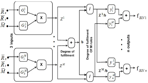
In the field of computational intelligence, neuro-fuzzy refers to combinations of artificial neural networks and fuzzy logic. This idea was proposed first by J. S. R. Jang [11]. Recently, this hybrid approach have received many attention from researchers whose dealing with non-linear control applications [8-9]. Moreover, neuro-fuzzy model is a hybrid intelligent system which combines the human-like reasoning style of fuzzy systems with the learning ability of neural networks. The main advantages of neuro-fuzzy system are: it interprets IF-THEN rules from input-output relations and it is an efficient universal-approximator. These are the main motivation for us to develop a control scheme of binary manipulator. In case of rigid body manipulator, the relation between inputs (forces and moments) and outputs (state of the actuators) in neuro-fuzzy model is explicitly shown in Fig. 2. Three normalized inputs (minimum value = 0 and maximum value = 1) and n binary outputs denote as input-output arrangement. Next, more explanation about the procedure of the fuzzy structure will be explained in Section 3.1 along with the learning procedure which is explored in Section 3.2. Additionally, the strategy to convert the real value of outputs fuzzy into binary value by using average threshold strategy can be seen in Section 3.3.

A. Fuzzy logic system: Takagi-Sugeno type MIMO

Neuro-fuzzy model as shown in Fig. 2 below is based on Gaussian membership functions (GMFs). It uses Takagi-Sugeno (TS) model (note: compare to Mamdani model and Pedrycs model, both linguistic fuzzy models that are focused on interpretability, a TS model is a precise fuzzy model that focused on accuracy and it has strongly connection between input and output). Moreover, a TS model is easy to interpret, and its outputs obtained from the networks are crisp outputs,

means directly compatible to the actuator’s states.

Figure 2. Takagi-Sugeno-type MIMO ( with input real and output binary) feedforward Neuro-Fuzzy network, no. input = 3, no. output = n-bit actuators,

no. membership function = M, training method: LMA

As shown in Fig.2, the Gaussian nodes to calculate the degree of membership of the numerical input values in the antecedent (IF part) fuzzy sets. The product nodes (×) represent the antecedent conjunction operator and the output of this node is the corresponding degree of fulfillment , with

After this, the division symbol (/), together with summation (+), join to make the normalized degree of fulfillment ( ⁄ ) of the corresponding rule. Then, the multiplication of ⁄ with the corresponding TS rule consequent (THEN part) is used as input to the last summation part (+) at the crisp output value which is directly compatible with the bi-state of the actuator arrays.

Furthermore, fuzzy model type TS-MIMO, with Gaussian membership functions (GMFs), product inference rule, and a weighted average defuzzifier can be defined as three layers feedforward network, as explained in (3.1a-3.1c) below: (see [5] for details).

∏ ( ) ( ) ( ( ) ) (3.1a)

(3.1b)

∑ (3.1c)

where ⁄ , and ∑

and is the output binary state of the j actuators(output prediction).

The corresponding rule from the above fuzzy logic system (FLS) can be written as

1 3

1 3

0 1 1 3 3

:

is

AND ... AND is

...

.

l l l

l l l l

j j j

j

R

IF x

G

x

G

THEN

x

x

y



W



W

 

W

(3.2)

where, with i = 1, 2, 3; are the 3 inputs, with j = 1, 2,

…, n; are its n outputs, and with i = 1, 2, 3 and l= 1, 2, …, n

are the Gaussian membership functions of form (3.1) with the corresponding mean and variance parameters and



_il

respectively and with l j

y as the output consequent of the _lth rule. It must be remembered that the Gaussian membership

functions

G

il actually represent linguistic terms such as low,

medium, high, very high, etc. The rules as written in (3.2) are known as Takagi-Sugeno rules.

Because of the neural network procedure (neuro) is implemented to the Takagi-Sugeno model, this figure represents a Takagi-Sugeno-type of MIMO (multi real-input multi binary-output) neuro-fuzzy network, where instead of the connection weights and the biases in neural network, we

have here the mean

c

_iland also the variance



_il parameters of Gaussian membership functions, along with the rules consequent l

ij l oj

W

W

,

parameters, as the equivalent adjustable parameters of the network. If all these parameters of NF network are properly selected by training mechanism, then the FLS can correctly approximate any nonlinear systems based on given data of inputs (forces, moments)-outputs(state of the actuators) pairs.

B. Levenberg Marquardt Algorithm (LMA) procedures

More detail of LMA equation, will be explained below. If a function

V

 

w

is to be minimized with respect to the

parameter vector w (these parameters are to be updated in

training algorithm) using Newton’s method [12], the updated parameter vector and are defined as:

 



V w



V

 

w w 

 ₂ 1

(3.3a)



k



w

 

k w

w 1   (3.3b)

In equation (3.3a), 2V

 

wis defined as the Hessian matrix and V

 

w is the gradient of V

 

w . If the function V

 

w is taken to be a SSE function as follows:

 

w

e

 

w

V

N r r









1 2

5

.

0

, (3.4)

then the gradient of

V

 

w

and the Hessian



2

V

 

w

are generally defined as:

 

w J

   

w ew V _ T _

 (3.5a)

 

w J

   

w J w e

 

w e

 

w

V _r N r r T 2 1

2 _{   }







(3.5b)

where, the Jacobian matrix

J

 

w

is as follows:

 

 

 

 

 

 

 

 

 

 

                                         p p p N N N N N N w w e w w e w w e w w e w w e w w e w w e w w e w w e w J       2 1 2 2 2 1 2 1 2 1 1 1 (3.5c)

From (3.5c), the dimension of the Jacobian matrix is

, where is the number of training samples and is the number of adjustable parameters in the network. For the Gauss-Newton method, the second term in (3.5b) is assumed to be zero. Therefore, the updated equations according to (3.3a) will be:

   



J w J w



J

   

w ew

w T   T 

 1

3.6a) Now let us see the Levenberg-Marquardt’s modifications of the Gauss-Newton method:

   



J w J w I



J

   

w ew

w T     T 

 1



(3.6b)

where, I is the identity matrix, and the parameter is multiplied or divided by some gain/factor whenever the iteration step increases or decreases the value of V

 

w .

Here, the updated version of (3.3a), can be seen on (3.6c) as follows:



k

  

w

k



J

   

w

J

w

I



J

   

w

e

w

w



1





T









1



T



(3.6c) It is important to know that for large



, the algorithm becomes the steepest descent algorithm with step size 1/



, and for small



, it becomes the Gauss-Newton method.

Furthermore, Xiaosong et.al [10] also proposed to add modified error index (MEI) term in order to improve training convergence. The corresponding gradient with MEI can now be defined by using a Jacobian matrix as:

 

   





 

avg





T

new

w

J

w

e

w

e

w

e

SSE











where e

 

w is the column vector of errors,

e

avg is the

average training error of each column, while



is a constant factor,  1 has to be chosen appropriately.

Now, the computation of Jacobian matrix can be performed as follows. The gradient

 

l

j

W

V

₀



can be written as:

  

  



j j



l l

j l

j

S

W

z

b

f

d

W

V















₀

/

₀

/

(3.8)

where,

f

j and

d

j are respectively the actual output and

desired output of the Takagi-Sugeno type MIMO neuro-fuzzy network. Now, by comparing (3.8) to (3.5a), where the gradient

 

w V

 is expressed as the transpose of the Jacobian matrix multiplied with the network's error vector, i.e.

 

w

J

   

w

e

w

V



T





(3.9)

the corresponding Jacobian matrix for the parameter l j

W₀ of the NF network can be written as:

 



 

_l

  

T _l T j

T l

j J W z b

W

J ₀  ₀  / (3.10)

where prediction error of NF network is written as:



j j



j f d

e   (3.11)

If the normalized prediction error on NF network is considered, then instead of equations (3.10), the corresponding Jacobian will be as follows:

 



 

l

  

T l T j T l

j J W z

W

J 0  0  (3.12)

This is because the normalized prediction error of the MIMO-NF network is



normalized





f

d



b

e

j



j



j

/

(3.13)

Similarly, Jacobian matrix itself for the parameter l ij

W of the

NF network can be written as:

 



 





 



T

i l T l ij T l

ij J W z b x

W

J   /  (3.14)

Also, by considering normalized prediction error from (3.11), equations (3.14) then become:

 



 

  

T

i l T l ij T l

ij

J

W

z

x

W

J







(3.15) Now, the Jacobian matrix computation of the remaining parameters

c

il and

l i



are performed by defining the terms

eqv

D

and

e

eqv as



m m



eqv

eqv

e

D

e

D

e

D

e

D

D







₁



₁



₂



₂









(3.16) Where,



l



j j j

D  y f and ej



fjdj



with j = 1, 2, .., m and the term e_eqv is such that it contributes the same amount of

sum squared error that can be obtained jointly by all the errors

j

e from the MIMO network. Therefore,



2 2 2



2 1 p m p p p

eqv e e e

e    (3.17)

Where, p = 1, 2, …, n; corresponding to n as number of training samples/data.

Now, by considering normalized equivalent error in (3.13), taking into account the equation (3.9), the transposed Jacobian matrix for the parameters

c

il and

l i



can be computed as:

 



 





  

l T

i l i i l eqv T l i T l

i J c D z x c

c

J  _2    /



2_ (3.18)

 



 





  

l T

i l i i l eqv T l i T l

i J D z x c

J   _2    2/ 3_ (3.19)

The above procedure describes actually layer by layer computation of Jacobian matrices for various parameters of neuro-fuzzy network (see [8] for details). Again, after finish all the Jacobian computation, back to the equation (3.6c) for updating the parameters. This updating procedure stops after achieving the maximum iteration or the minimum error, with setting parameters: maximum iterations = 500, momentum constant = 0.005, oscillation control WF = 0.5%, constant factor



= 0.0007.

In addition to LMA procedure, we proposed a simple optimization procedure in order to find the tuning parameters on neuro-fuzzy systems, known as randomized Hill Climbing procedure (HC). This procedure is a local search algorithm and tries to find the best local minimum from huge stochastic procedure, by permitting the best training parameters that minimize the error function (RMSE) and neglecting the others. The results of using HC can be shown latter in Table III.

The following steps of HC are carried out:

a. Run the loop: No. membership function form 2-15 (M) b. Run the loop: No. experiment of each initial parameters

= 100

c. Run the loop: No. of iteration, each experiment has iteration from 50 to 500

d. Calculate training output and find the suitable prediction model ̂

e. Save the parameters after step d completed. If the next iteration produce better result, replace the old parameters, otherwise the new parameters are neglected. f. Determine the forces and moments prediction and

calculate the prediction performance error

g. Early stopping criteria[6]: Terminate the program if criteria are satisfy in step f

h. Repeat again step a if needed and save the best parameters (time computing in 2 weeks).

IV. EXPERIMENT PROCEDURES AND RESULTS

By using neuro-fuzzy network that shown in Fig.2, we propose two experiments for modeling and testing the rigid body manipulator as follows:

1. Input forces and moments from fix angle

There are 3 equivalent actuator model (4-bit, 8-bit and 12-bit actuators) and testing data taken from equivalent 15 actuators. The results of this experiment are shown in Table II and Fig.3 .

2. Input forces and moments from variety angle (10, 20, 30, 40, 50, 60, 70).

TABLE II. 1ST

EXPERIMENT WITH 4-BIT,8-BIT AND 12-BIT

PERFORMANCES (AFTER 2 WEEKS LEARNING)

Descriptions 4-bit Actuators

8-bit Actuators

12-bit Actuators RMSE RX 1.6862 1.2726 0.8440

RMSE RY 4.2326 2.5840 2.0005

RMSE MR 34.9179 27.3226 20.0735

% Error RX 17.20 13.99 9.19

% Error RY 24.30 13.17 9.84

% Error MR 15.51 12.56 8.78

Procedure for 1st experiment according to Fig.2 can be explained with several steps:

a. Derive the equilibrium equations (2.1 to 2.7) using 4-bit, 8-bit and 12-bit actuator system with alpha=20 deg and put the result in input output arrays

̅̅̅̅ ̅̅̅̅ ̅ ̅̅̅̅̅̅ ]

b. Calculate training output of the state actuators ̂ c. Generate testing data from equivalent system 15-bit with

50 data set.

d. Determine binary prediction ̂

e. Calculate again forces and moments model using ̂ (for validation)

f. Determine performance error

g. Repeat step a to f using search method (Hill Climbing) for finding the best parameter that give minimum error in two weeks.

Figure 3. Moment model and testing with single deg and actuators = 4-bit, 8-bit, 12-bit with data testing 15-bit

Moreover, Fig.3 demonstrates the performance of the neuro-fuzzy model using 3 inputs with orientation angle 20 (deg). The dashed lines are the validation of forces and moments of the model when 50 sets of testing data from equivalent system 15 actuators (black-solid lines) are entered the trained model of 4-bit, 8-bit and 12-bit. Furthermore, Table II shows the performance results after 2 weeks learning time. We can see that 12-bit model can bring the performance RMSE down to 10%, as error minimum required.

TABLE III. 2ND

EXPERIMENTS,12-BIT PERFORMANCES

No. Actuators = 12, Optimized Parameters Alpha learning = 10,20,30,40,50,60,70, with 100 data testing

from alpha 17, 25, 35, 45

Description Learning after 1 weeks

Learning after 2 weeks

RMSE RX 1.7455 1.3499

RMSE RY 2.6064 2.2929

RMSE MR 22.8522 17.0078

% Error RX 13.96 11.69

% Error RY 12.47 10.77

% Error MR 12.74 9.84

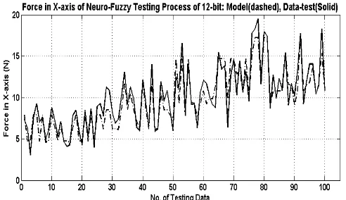
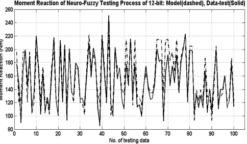
Procedure for 2nd experiment according to Fig.2is similar with the first experiment but we used several learning orientation angle. Here, 12-bit actuators are chosen as the optimized number of actuator arrays. The result of 1 week and 2 weeks computing time can be seen on Table III as well as some figures on the validation using 100 data test from the 12-bit with angle 17, 25, 35, 45 (25 data from each angle).

Figure 4. Force X-axis validation of the neuro-fuzzy 12-bit model, using data testing 12-bit from angle α (17, 25, 35, 45) after 2 weeks learning

Figure 6. Moments validation of the neuro-fuzzy 12-bit model, using data testing 12-bit from angle α (17, 25, 35, 45) after 2 weeks learning

Table III shows the performance result of the input model of 12-bit with alpha from 10, 20, 30, 40, 50, 60 and 70, with its testing data from 12-bit with alpha 17, 25, 35, and 45. In addition, Figs. 4-6 illustrate the performance of the neuro-fuzzy model using 3 inputs and 12-bit outputs of forces and moments, to keep the rigid body in equilibrium position, when 100 sets of testing data(random testing) are entered the NF 12-bit model. The results of the model validation feature error average validation RMSE around 13% after 1 week computation and RMSE around 10% after 2 weeks computation. These results give the improve of using randomized Hill Climbing in the learning computation.

V. CONCLUSION

In this paper, a neuro-fuzzy network type TS MIMO have been presented for prediction the states of the actuators with the input networks are forces and moments of rigid body manipulator (parallel configuration, in 2D) that already known before. It has been demonstrated that neuro-fuzzy network and trained with Levenberg-Marquardt algorithm, is very efficient to find performance error around 10% in off-line learning and with around hundred testing data. The neuro-fuzzy model also proposed the number of actuators = 12 as the minimum actuators that should be put in the rigid body system. From our first results, it can be inferred that this model has flexibility to test the trained model with any orientation inputs.

For the next issue, we would like to use the efficient NF to more complex geometry of binary manipulators such as robot

manipulator with bi-state actuator arrays for rehabilitation purpose.

Instead of neuro-fuzzy, other approximator method, such as recurrent neural network (RNN) can be used in these problems. Theoretically, the biologically inspired solution, such as RNN method can bring the performance error less than neuro-fuzzy, although it uses a huge computation time.

REFERENCES

[1] G. S. Chirikjian, A binary paradigm for robotic manipulators, in: Proc. IEEE Int. Conf. On Robotics and Automation, San Diego, CA, pp. 3063– 3069 (1994).

[2] I. Ebert-Uphoff and G. S. Chirikjian, Efficient workspace generation for binary manipulators with many actuators, J. Robotic Syst. 12(6), 383– 400 (1995).

[3] I. Ebert-Uphoff, On the development of discretely-actuated hybrid-serial–parallel manipulators, PhD Dissertation, Johns Hopkins University (1997).

[4] J. Suthakorn and G. S. Chirikjian, “A new inverse kinematics algorithm for binary manipulators with many actuators,” Adv. Robot., vol. 15, no. 2, pp. 225–244, 2001.

[5] A.K. Palit, R Babuška, “Efficient training algorithm for Takagi-Sugeno type Neuro-Fuzzy network,” Proc. of FUZZ-IEEE, Melbourne, Australia, vol. 3: 1538-1543, (2001)

[6] A.K. Palit, D. Popovic, “Nonlinear combination of forecasts using ANN, FL and NF approaches,” FUZZ-IEEE, 2:566-571, (2002).

[7] A. K. Palit, G. Doeding, W. Anheier, and D. Popovic, “Backpropagation based training algorithm for Takagi-Sugeno-type MIMO neuro-fuzzy network to forecast electrical load time series,” Proc. Of Fuzz-IEEE, Honolulu, Hawai, vol. 1:86-91, (2002)

[8] A. K. Palit, D. Popovic, “Computational Intelligence in Time Series Forecasting, Theory and Engineering Applications”, Springer, (2005). [9] F. Pasila, A.K. Palit, G. Thiele, “Neuro-Fuzzy Approaches for Electrical

Load forecasting using additional Moving Average Window Data Filter on Takagi-Sugeno Type MISO Network” Journal of Advanced Computational Intelligence & Intelligent Informatics, JACIII 12(4): 361-369, Fuji Technology Press Ltd, Japan, (2008)

[10] D. Xiaosong, D. Popovic, G. Schulz-Ekloff, Oscillation resisting in the learning of Backpropagation neural networks, Proc. of 3rd IFAC/IFIP, Ostend, Belgium, (1995)

[11] J.S.R. Jang, “ANFIS: Adaptive network Based Fuzzy Inference System,” IEEE Trans. On SMC., 23(3):665-685, (1993)