DEM GENERATION FROM CLOSE-RANGE PHOTOGRAMMETRY USING
EXTENDED PYTHON PHOTOGRAMMETRY TOOLBOX
A. A. Belmonte, M. M. P. Biong, E. G. Macatulad *
Department of Geodetic Engineering, College of Engineering, University of the Philippines, Diliman, Quezon City, Philippines - (aabelmonte1, mpbiong, egmacatulad)@up.edu.ph
KEY WORDS: Digital Elevation Model, DEM, terrestrial close-range photogrammetry, Free Open Source Software (FOSS), Python Photogrammetry Toolbox, PPT
ABSTRACT:
Digital elevation models (DEMs) are widely used raster data for different applications concerning terrain, such as for flood modelling, viewshed analysis, mining, land development, engineering design projects, to name a few. DEMs can be obtained through various methods, including topographic survey, LiDAR or photogrammetry, and internet sources. Terrestrial close-range photogrammetry is one of the alternative methods to produce DEMs through the processing of images using photogrammetry software. There are already powerful photogrammetry software that are commercially-available and can produce high-accuracy DEMs. However, this entails corresponding cost. Although, some of these software have free or demo trials, these trials have limits in their usable features and usage time. One alternative is the use of free and open-source software (FOSS), such as the Python Photogrammetry Toolbox (PPT), which provides an interface for performing photogrammetric processes implemented through python script. For relatively small areas such as in mining or construction excavation, a relatively inexpensive, fast and accurate method would be advantageous. In this study, PPT was used to generate 3D point cloud data from images of an open pit excavation. The PPT was extended to add an algorithm converting the generated point cloud data into a usable DEM.
1. INTRODUCTION
1.1 Background of the study
Mining and many other land development projects rely heavily on accurate topographic maps for most of its activities. For larger and complex projects, extensive technologies such as the LiDAR or aerial photogrammetry are employed. These technologies are expensive and thus are used only on the start and end of project. For small-scale projects, traditional surveying methods, such as the use of a total station are employed in generating reference topographic maps. The traditional survey methods produce terrain models with accuracies limited by the number of observed points (Patikova, 2012). Thus, more survey points are necessary for better accuracy, but would mean additional time and cost.
Terrestrial photogrammetry deals with photographs taken with cameras located on the surface of the earth. The term Close-Range Photogrammetry or CRP is generally used for terrestrial photographs having object distances about 300 meters (Wolf, et al., 2014). This methodology is one alternative to produce DEMs through the processing of images using photogrammetry software. Luhmann (2011) relates that CRP is applicable to objects ranging from 1 m to 200 m in size (Luhmann, 2011). Aside from the distinctive speed of data collection, employing photogrammetric methods also deliver results within a relatively short period of time, achieve results of acceptable accuracy and provide instant documentation via the captured images. CRP, in particular, provides a low-cost, rapid, yet accurate method of object and surface modelling which makes it an effective method of topographic surveying for small scale earthwork operations and site monitoring that requires frequent implementation.
Powerful photogrammetry processing is possible using many cross-platform software available with free trials such as Pix4D, Photomodeler and Agisoft, that can generate high-quality digital elevation models. However, most of these trials are extremely limited in terms of usable features and usage period. Many FOSS photogrammetry software are also available that can generate high-quality 3D models such as the Python Photogrammetry Toolbox (PPT). Unlike most photogrammetry software, PPT has a minimal size and, being a FOSS, has a very transparent workflow. Unfortunately, these models are usually described in arbitrary coordinates and cannot readily be used for DEM generation. Thus in this study, PPT was extended to add an algorithm converting the generated point cloud data into a usable DEM.
1.2 Objectives
Studies on the utilization of PPT, particularly in terrestrial photogrammetry for the generation of DEMs are still few. Thus, this study aims to assess the efficiency of the PPT in generating relatively accurate dense 3D point cloud for the production of DEMs. An algorithm is developed that extends the PPT functionalities to produce raster DEMs. The vertical accuracy of the generated DEMs will be assessed based on an existing DEM of the study area.
1.3 Study Area
The selected study area is the on-going excavation work for the foundation of the proposed faculty and staff housing of the University of the Philippines located in E. Jacinto St. Diliman, Quezon City. The area has an approximate total area of 0.40 hectares. Three buildings are planned to be constructed in this area. Figures 1(a) to (c) show different site details of the study area.
(a) (b)
(
(c)
Figure 1. Details of the study area: (a)sample view of the site; (b) site plan proclamation sign; and (c) site vicinity map from
Google Maps
The site is divided into three open-pit excavations corresponding to the planned buildings, as seen in the aerial photo of the site shown in Figure 2.
Figure 2. Aerial photo of the study area showing the three planned building sites (A, B, and C)
1.4 Assumptions and Limitations
Further study on different types or larger extent of areas is yet to be determined. It is also assumed that construction sites have their own local project controls for their own purposes.
The processing speed and capability of the PPT and its extensions or modifications used in the study is only implemented on two workstations: an Asus N550JK-CN309H and Lenovo G470. No modifications were made on the original PPT code but an additional Python script was utilized to process its outputs into DEMs.
Meshlab was used to visualize the .ply outputs of PPT. The output DEM is a raster in ESRI-ASCII format and for visualization, ArcMap was used to convert the ASCII raster into TIFF. This study only considers evaluating the vertical accuracy of the DEMs.
2. MATERIALS AND METHODS
Shown in Figure 3 is the six-step general methodology of this study, which is adapted from the four steps for close-range photogrammetry projects described in (Barnes, et al., 2014).
Figure 3. General methodology of the study
2.1 Project Planning
Project planning includes the development of strategies for the selected site or object, selection of the equipment and software to be used, calibration of the equipment (if necessary), and acquisition of any required permissions.
Visiting the site or reviewing the subject area and taking various test shots for study prior to planning is recommended. Planning all the camera stations and control points, as well as the time needed for site preparation should be done thoroughly after the reconnaissance. All possible working conditions and other site specifics such as: weather, visibility, sun or shadows, equipment, assistance, safety regulations, and legal responsibilities are also considered as recommended in (ISPRS Commission V, 2010).
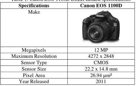
A Canon EOS 1100D DSLR camera is used for the acquisition of the images. The EOS 1100D is a high-performance DSLR camera that features a fine-detail CMOS sensor with approximately 12.2 effective megapixels. (Canon Inc., 2011). Further specifications of the camera used are listed in Table 1.
Table 1. Canon EOS 1100D DSLR camera specifications
Specifications Canon EOS 1100D
Make
Megapixels 12 MP
Maximum Resolution 4272 x 2848
Sensor Type CMOS
Sensor Size 22.2 x 14.8 mm
Pixel Area 26.94 µm²
Year Released 2011
The Python Photogrammetry Toolbox accepts any image datasets provided that the camera sensor width is known to the user. The Canon EOS 1100 DSLR camera is selected due to its capable sensor size and availability. Based on the literature, Study Area
DSLR cameras tend to give optimum results than those of compact digital cameras due to the fact that they are equipped with more advanced and higher quality lenses than digital cameras (ISPRS Commission V, 2010). Since PPT will be used for processing, there is no need for external camera calibration. PPT uses Bundler, a structure-from-motion system for unordered images which only requires the user the image network of geometrically coherent pictures and the internal camera parameters such as focal length or camera sensor size.
2.2 Field Set-up and Control Survey
Collecting images for a photogrammetric project requires particular techniques so that the processing part will be handled seamlessly by the software. Providing external control information to a photogrammetric project is important to position the model relative to a reference frame. If the photogrammetric model need to be situated in an existing reference frame, then sufficient external references defined in this frame should be integrated into the project. For the three excavation sites previously shown in Figure 2, a control survey utilizing a total station instrument was first performed to establish four (4) local ground control points (GCPs) at the corners outside of the excavation sites based on a reference baseline with arbitrarily set coordinates and azimuth.
2.3 Image Acquisition
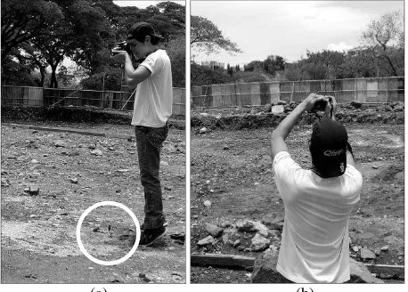
Image acquisition involves taking pictures of the area, with the condition that GCPs must be occupied while taking pictures. It is important that the camera axis is directed towards the center when taking photos and the camera stations are placed at intervals no greater than 3 meters along the perimeter of the site. For areas with high obstruction or noise, smaller intervals are recommended. There are no strict guidelines in taking pictures as long as the image quality is good. For this study, two photos per camera station were done: (1) directly over the station and centered towards the subject, and (2) a few steps back to ensure that the edge or wall of the excavation for both the near and far sides of the area are visible.
Figure 3 shows a sample image acquisition methodology at one GCP location.
(a) (b)
Figure 3. Site image acquisition: (a) camera over a GCP, using a plumb bob; and (b) image taken a few steps back from GCP
At least one image was captured wherein the camera was stationed along the same x-y coordinates of each GCP. This coincidence along the horizontal plane was ensured with the use of a plumb-bob attached to the camera. The length of the string
attaching the plumb bob to the camera was fixed and measured so as to define the z-coordinates of the camera during image digital processing which involves adjustments and manipulations to the various image properties. An important note is to never manipulate the image dimensions in any way. To extract 3D points from 2D images, it is essential to perform a triangulation with at least two overlapping images or what we call a stereo pair. When more than two images are used in a triangulation, we denote this group of images as a „block‟. In order to perform a triangulation of the entire block, known as the bundle block adjustment, the user must measure a sufficient number of tie, control, and check points throughout the block. Adding constraints on certain sets of points may help to enforce angular, linear, and/or planar properties.
2.5 Python Installation
Python is a dynamic and open source programming language that lets its user work quickly and integrates systems more effectively (Python Software Foundation, 2015). It has a simple syntax that is natural to read and easy to write. Its ingenuity lead to many applications through its numerous third party modules and libraries such as the Python Photogrammetry Toolbox (PPT). PPT requires Python and its associated packages to run its processes. Table 2 describes the required software readily available online and could be easily installed.
Table 2. Python Installation requirements: file types and file size
PyQt4 was used for the development of PPT-GUI, as well as the GUI for the algorithm extension developed. Pillow is the friendly edited version of the Python Imaging Library or PIL, which is a free library for the Python programming language that adds image processing capabilities. NumPy is the fundamental package for scientific computing with Python and allows for the creation and manipulation of N-dimensional arrays. The SciPy Stack is a collection of open source software that are widely used for scientific computing in Python. The SciPy library is one of the core packages that make up the SciPy stack which provides many simplified yet highly efficient numerical routines such as the interpolate module used in this study.
2.6 PPT Processing
The Python Photogrammetry Toolbox (PPT) is a free/libre, open-source and cross-platform photogrammetry software originally developed by the Arc-Team, Pierre Moulon and Alessandro Bezzi in September 2010. The toolbox is composed of python scripts that automate the 3D reconstruction process from a set of pictures and have been used for various purposes such as 3D forensic reconstruction, 3D modelling of cultural The International Archives of the Photogrammetry, Remote Sensing and Spatial Information Sciences, Volume XLII-4/W5, 2017
heritage sites, and 3D modelling for archaeological studies. The processes performed in PPT can be simplified into two parts: camera pose estimation/calibration and dense point cloud computation. Open-source software are employed to perform these intensive computational parts, namely: Bundler for the calibration and CMVS/PMVS for the dense reconstruction.
2.7 Run Bundler
Reconstruction of a scene from images poses problems such as correspondences between pairs of images and calculating the required geometries for the common coordinate system among the image sequence. Structure from Motion (SfM) and Image-based Modelling (IBM) are solutions to the 3D reconstruction problem (Moulon and Bezzi, 2011). SfM is the process of automating the retrieval of camera orientation parameters beside the 3D positions of the tie points by analyzing a sequence of images and IBM is the process of creating 3D models from 2D images (Alsadik, 2014).
SIFT is an algorithm established by David Lowe (2004) that detect and describe features in images. The algorithm was published in 1999 and has since been used in numerous applications in the field of computer vision. The Python Photogrammetry Toolbox uses this algorithm via Bundler. The algorithm is patented in the US under the ownership of the University of British Columbia (Lowe, 2004).
Despite its popularity, the original SIFT implementation is available only in binary format. VLFEAT, an open and portable library of computer vision algorithms, provides an open-source implementation of SIFT.
Bundler is a structure-from-motion (SfM) system for unordered image collection (Snavely 2009) that is utilized by the PPT. The camera positions are defined by using the relative geometry between the cameras. Bundler outputs the following: a bundle file which contains the parameters needed to define the camera and scene geometry and a .ply file which contains the reconstructed camera and point orientations. Bundler performs the camera pose estimation processing. Run Bundler allows the user to specify the directory containing the input images, the feature extractor and the image size or scale.
2.8 Run CMVS/PMVS or PMVS2
Multiple View Stereovision (MVS) consists of mapping image pixel into a dense 3D point cloud or mesh (Moulon and Bezzi, 2008). It uses multiple images in order to reduce ambiguities in pixel locations and to produce accurate estimates of the 3D position of each pixel. Most multi-view stereo algorithms, however, cannot handle well large numbers of input images due to limitations in computational and memory resources. PPT uses the Clustering Views for Multi-view Stereo software (CMVS) which takes the output of a SfM software as input then decomposes the input images into a set of image clusters of manageable size (Furukawa and Ponce, 2010), thus allowing a less memory-extensive computer processing.
The Patch Multi-view Stereo (PMVS) which is included in the CMVS package uses a seed growing strategy in its reconstruction approach. It finds corresponding patches between images and locally expands the region by an iterative expansion and filtering steps in order to remove bad correspondences. Such an approach finds additional correspondences that were rejected or not found at the image matching phase step (Moulon and Bezzi, 2008).
CMVS performs the point densification using the Run Bundler outputs and the input images. It uses Bundle2PMVS and RadialUndistort to convert the bundler outputs into CMVS/PMVS format. The users can choose between CMVS and PMVS; for larger datasets, however, CMVS is recommended.
2.9 Post-Processing of PPT Output
The algorithm developed was annexed to the original PPT code and referred to as CMVS Post-Process. This algorithm imports some of the CMVS output files as well as a user defined input file to construct a DEM in ESRI ASCII format raster file based on the PPT-generated point cloud. The implementation of this algorithm is simplified via the PyQT GUI used in PPT.
The 3D coordinates of the generated point cloud from PPT are consolidated in one single PLT file which are then scaled, oriented and translated to the proper 3D location. This is done by extracting the images specified in a user-inputted text file of which the 3D ground coordinates of the camera centers are obtained. These coordinates will serve as the ground controls for the subsequent least squares adjustment computation to perform the 3D conformal coordinate transformation of the 3D point cloud defined by 7 parameters: 3 translations Tx, Ty, Tz to
the origin of the target coordinate system, 3 rotation angles ω, φ, κ about the XYZ and one scaling factor m for Equation (1):
(1)
where r is a function of the rotation angles ω, φ, κ.
Included in the CMVS Post-Process algorithm is the computation of a General Least Squares Adjustment (GLSA) to solve for the 3D Conformal Coordinate Transformation (3DCCT) parameters. Based on the solved 3DCCT parameters, the algorithm then performs 3DCCT on all coordinates contained in the consolidated PLY file. These are then used to generate the DEMs as outputs.
The cell values of the DEM output raster is mapped out to the original input coordinate system to assign a value to each output cell. Techniques have been used to define the output value depending on where the point falls relative to the center of cells of the input raster and the values associated with these cells. Among of these techniques are Nearest Neighbor, Linear Interpolation, and Cubic Convolution. These image resampling techniques are also same to the gridding interpolation method SciPy uses. Each of these techniques assigns values to the output differently. Thus, the values assigned to the cells of an output raster may differ according to the technique used (ESRI, 2016). Nearest neighbor returns the value at the data point closest to the point of interpolation; linear interpolation tessellate the input point set to n-dimensional simplices, and interpolate linearly on each simplex; and cubic convolution returns the value determined from a cubic spline. For the initial tests in this study, the aforementioned three techniques are implemented.
2.10DEM Validation
Aside from the ground controls used for the 3DCCT, validation points were also established during the control survey. 33 points for Site A and 21 points for Site B. Site C was not included due to inaccessibility of the area during the control point survey. The International Archives of the Photogrammetry, Remote Sensing and Spatial Information Sciences, Volume XLII-4/W5, 2017
The ground controls were used to assess the accuracy of the output DEMs.
The elevation values from the generated DEMs of sites A and B corresponding to the ground validation points were collected and tabulated from which the root-mean-square error (RMSE) was computed by the formula (Luhmann, et al., 2011):
(2)
where Xi is the elevation of the validation points, is the
elevation derived from the DEMs, and n is the number of validation points. The RMSE is equal to the empirical standard deviation of the model (Luhmann, et al., 2011).
3. RESULTS AND DISCUSSIONS
3.1 Initial Tests
Preliminary tests were done prior to the field photo documentation to check the efficiency of the PPT in creating high fidelity point clouds. Various tests were performed using varying-size models to evaluate the processing speed of the software and the qualities of the outputs at varying input parameters. In line with the research objectives, the following values were established as the default PPT input parameters based on the results of the preliminary tests:
Feature Extractor : SIFT implementation by VlFeat Max Photo Width : 2000 pixels
Multi-view stereovision : CMVS
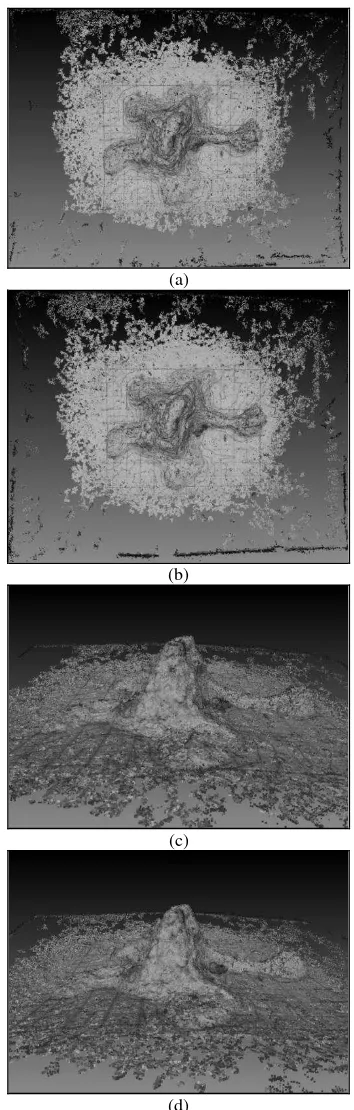
The first test was performed to compare the outputs of using SIFT by David G. Lowe (2004) and SIFT by VlFeat as feature extractors. A maximum photo width of 2000 pixels was used for the PPT processing. PMVS2 was used for point densification. The test was performed to compare the features detected by the two feature extractors. For this test, a terrain model with a relatively rough appearance was used as the sample model object to also test the efficacy of the feature extractors to detect features in coarse textures.
The results presented in Table 2 show that the two extractors are able to generate almost the same numbers of 3D points. Upon visual inspection via Meshlab, the resulting 3D point clouds differ in terms of scale and orientation but are able to describe the same areas on the objects. This validates that the original SIFT by Lowe and the OS implementation are “output equivalents”. This is also seen in the Figures 4(a), (b), (c) and (d). However, there is a huge disparity between the processing times of the two feature extractors. For the given dataset, feature extraction using SIFT by VlFeat consumed more than twice the time than SIFT by Lowe. Nevertheless, it still affirms that the SIFT implementation by VLFEAT indeed provides an effective albeit slower alternative as feature extractor versus the original SIFT implementation by David G. Lowe. Using the VlFeat implementation also protects future users from the infringement of the copyright attached to the original SIFT by David G. Lowe.
Table 3. Output details of SFT by Lowe and SIFT by VlFeat
Detail Lowe VlFeat
Bundler Output Size (KB) 761 2,346 CMVS Output Size (KB) 17450 18,714
# of points/vertices 260,151 282,730 Processing Time (minutes) 20 50
(a)
(b)
(c)
(d)
Figure 4: Sample views of the outputs using (a) SIFT by Lowe (2004), Top view; (b) SIFT by VlFeat, Top view; (c) SIFT by Lowe (2004), Front view; and (d) SIFT by VlFeat, Front view;
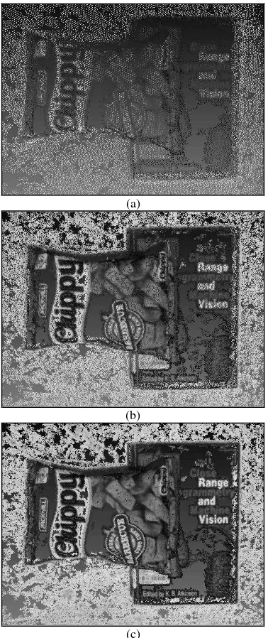
The second test was performed to compare the outputs of using different values for the maximum photo width. SIFT by VlFeat was used for feature extraction. PMVS2 was used for point densification. A different object with more geometrical features was used as model for easier comparison. Figures 5(a), (b), and (c) show the generated 3D point cloud using different maximum photo width. Upon visual inspection, it can be seen that varying the values for maximum photo width resulted to a significant difference in the densities of the output point clouds.
(a)
(b)
(c)
Figure 5: Comparison of 3D point cloud outputs from varying the values for maximum photo width: (a) 1200-pixel output; (b)
2000-pixel output; (c) 2700-pixel output
Results shows that varying the values for maximum photo width resulted to a significant difference in the densities of the output point clouds. The results presented in Table 4 indicate that an increase in image width corresponded to an increase in number of generated points. This is expected since a bigger input image equates to a bigger number of input pixels which, by logic, should also equate to a denser output.
Table 4. Test results of varying maximum photo width
Detail 1200 2000 2700
Bundler Output Size (KB) 757 844 756 CMVS Output Size (KB) 3,310 9,720 15,910
# of points/vertices 47,922 146,009 241,156 Processing Time (minutes) 10 32 55
Additionally, there is a linear relationship between the photo width and the processing time and number of generated points
at an R2 value of 0.9974 and 0.9991, respectively. This linearity indicates that there is no single most efficient value for the photo width since there is direct proportionality between the value and the processing time. The optimal value will depend on the desired density for the point cloud and will be at the discretion of the user. For the given data set, it was found out that a minimum photo width of 600 pixels was sufficient in creating an identifiable dense point cloud.
However, for larger model objects i.e. excavation sites, it was found that using 1200 pixels as photo width produced significant amounts of noise pixels. After further tests, it was suggested that 2000 pixels be used as compromise between processing time and output quality. Table 5 shows the results of these tests.
Table 5. Output qualities from varying photo width. Photos
Width
Processing Time (minutes)
# of
points/vertices Quality
1200 56 305761 incomplete
1400 49 396362 poor
1600 113 651046 moderate
1800 132 894206 acceptable
2000 203 1107498 fair
The third test was performed to compare the outputs of using CMVS and PMVS2 for point densification. However, the two are essentially the same except that CMVS was developed as a solution to the problems encountered in PMVS2. Using directly PMVS2 (without CMVS) with numerous images as input often results in the software crashing due to hardware limitations. For the Lenovo G470 with 500 GB DDRAM, a maximum of 50 images at 2000 pixels image width can be processed in PMVS2 (without CMVS) although a higher number of images can be processed using lower photo width. CMVS or clustering views for multi-view stereo processes these images by separate clusters instead of in a single batch. This partition decreases the workload for the processor for a given set thus allowing for a greater number of input images. Furthermore, using CMVS also results to a greater number of generated points.
However, CMVS generally consumes a longer processing time compared to PMVS2 (without CMVS). The user can shorten the processing time by increasing the number of images per cluster. Also, using greater number of images per cluster generally results to a sparser point cloud although this does not really equate to a lower quality 3D model, as seen in the output models. Upon visual inspection of the outputs, no distinct point cloud was identified as the “best” since the differences among the 4 models are too random even though the lowest image per cluster has the most generated points.
Therefore, it was concluded that it can be the users‟ discretion on what number of images will be used per cluster. To proceed with this study, the decision was that the denser point cloud is better and the default value at 10 images per cluster will be used. An actual excavation site was used as model object since smaller models only require few images.
3.2 DEM Generation Dense 3D Point Cloud Generation
The image datasets for sites A, B and C were then processed in the Python Photogrammetry Toolbox to generate a 3D point cloud using the input parameters discussed in Section 4.1. Table 6 shows a summary of the PPT outputs for the three sites. The International Archives of the Photogrammetry, Remote Sensing and Spatial Information Sciences, Volume XLII-4/W5, 2017
Table 6. Summary of PPT processing for all of the sites
Detail Site A Site B Site C
Processing Time 3h47m 4h30m 4h56m
Images per Cluster 15 20 10
Processed / Input 72/74 71/79 78/78 Generated Points 1,013,819 564,938 1,554,638
Output Quality Good Fair Poor
The developed CMVS Post Process algorithm was used to generate four (4) ESRI ASCII raster files containing the following information: elevation, red values, green values and blue values. The elevation raster can be converted into a TIFF file using ArcGIS to generate a digital elevation model. The red, green and blue values raster can be converted into a TIFF file to generate an RGB visualization of the area.
The algorithm allows the user to specify the raster cell width, the interpolation method as well as the output type. It gives three options for interpolation method, namely: Nearest Neighbor (NN), Linear Interpolation (LI) and Cubic Convolution (2DCC). For output type, it gives four options, namely: Elevation, Red Values, Green Values and Blue Values. The algorithm first imports the transformed CMVS output as the unstructured data. The algorithm then constructs a grid with intervals equal to the specified cell width and uses the unstructured data to interpolate for the values at each grid cell. Figures 6(a), (b) and (c) show the DEM produced using the three gridding techniques.
(a)
(b)
Figure 6. DEM result of Site A using (a) Nearest Neighbor; (b) Linear Interpolation; and (c) Cubic Convolution
The size of the grid is determined by the extents of the coordinates of the ground control points. For this study, 1cm was set as the default raster cell width, since the software usually crashes at less than 1cm. Table 7 describes the sample outputs of the different interpolation methods used in the generation of DEM for the Site A and B inputs.
Table 7. Processing time and output size of the DEMs summary
Site Interpolation Method
Processing Time (s)
Output Size (KB)
Site A
NN 476.8 109,608
LI 687.1 108,397
2DCC 713.6 107,563
Site B
NN 564.9 100,658
LI 395.4 100,653
2DCC 431.1 100,561
Results show that using Nearest Neighbor as interpolation method results in the least processing time. It also generated the highest output size. However, the difference in output size pales in comparison to the disparity on processing speed. Similar trends were noted in the results after processing the other sites.
3.3 Data Validation
Applying the root-mean-square error (RMSE) as discussed in section 2.6, the output RMSEs for the resulting DEMs using the three gridding methods were computed, summarized in Table 8.
Table 8. Summary of RMSE values for Site A and Site B DEMs
Site NN LI 2DCC
Site A 0.045454085 0.039003228 0.048366951
Site B 0.067141218 0.064736672 0.092858247
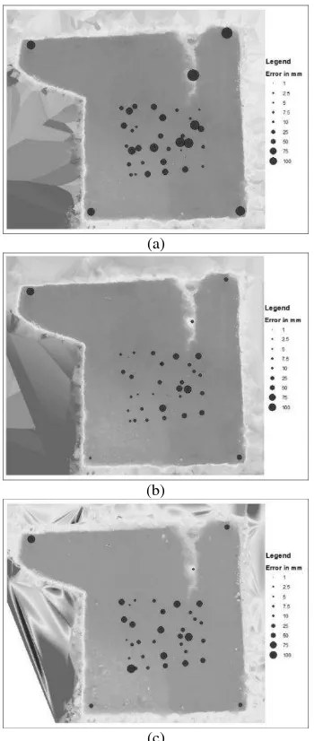
As seen in Table 8 above, for Site A, the linear interpolation gridding method produced the lowest RMSE value. This is also true for Site B, although the RMSE for linear interpolation in Site B is almost twice that of Site A. On the other hand, the highest RMSE value is for Site B, using the Cubic Convolution gridding method. These differences in values are possibly due to the distribution of the established control points.
Figures 8 and 9 show the distribution of RMSE of the generated DEMs for Site A and B using the three gridding methods. The International Archives of the Photogrammetry, Remote Sensing and Spatial Information Sciences, Volume XLII-4/W5, 2017
(a)
(b)
(c)
Figure 8. RMSE of the generated DEMs for Site A using (a) Nearest Neighbor; (b) Linear Interpolation; and (c) Cubic
Convolution
(a)
(b)
(c)
Figure 9. RMSE of the generated DEMs for Site B using (a) Nearest Neighbor; (b) Linear Interpolation; and (c) Cubic
Convolution
4. CONCLUSIONS AND RECOMMENDATIONS
4.1 Conclusions
The utilization of the Python Photogrammetry Toolbox (PPT) in terrestrial close-range photogrammetry presents an alternative to other costly methods for DEM generation. The PLY file outputs derived from PPT can be utilized to generate an accurate DEM with RMSE as low as 0.039 meters using linear interpolation as gridding method. The PLY files can also be used to create an interpolated DEM for red, green and blue values which can be merged to create an image as substitute to photo mosaics.
The DEMs produced could be used in various applications such as volume computation and surface representation. This technology could be the answer to the time-consuming process of obtaining high-accuracy terrain information. Accuracy at a single point can be up to centimeter level and is sufficient in the case of open pit excavations. The relative accuracy of 3D points derived from terrestrial photogrammetry is better than those derived from terrestrial measurements because of the higher number of points generated, which is able to represent the terrain well.
4.2 Recommendations
In pre-processing of images, manually increasing the contrast prior to PPT processing may be explored, which could further improve the accuracy of generated results. The use of faster feature extractors such as SURF and SIFT-GPU is also recommended. Manipulation of the default CMVS processing parameters can also supposedly significantly speed up the computation (Furukawa and Ponce, 2010). Addition of other function to the extended PPT, such as for area and volume computations, or further raster development processes using The International Archives of the Photogrammetry, Remote Sensing and Spatial Information Sciences, Volume XLII-4/W5, 2017
GDAL (Geospatial Data Abstraction Library) are some of the possible modifications that could be implemented. Also, to further assess the efficiency of the extended PPT, comparison of results obtained from processing the images using the commercial software such as Pix4D or Agisoft Photoscan with that of the PPT is recommended for future work.
ACKNOWLEDGEMENTS
Aerial photo courtesy of Engr. Christian Terence Almonte, as assisted by Engr. Mark Sueden Lyle Magtalas and Engr. Julius Caezar Aves of Phil-LiDAR Project 1 - PARMAP.
REFERENCES
Alsadik, B., 2014. Guided Close Range Photogrammetry for 3D Modelling of Cultural Heritage Sites. University of Twente Faculty of Geo-Information Science and Earth Observation, Enshende, The Netherlands, pp. 13-20.
Barnes, A., Simon, K., & Wiewel, A., 2014. From photos to models: Strategies for using digital photogrammetry in your project. [Online] University of Arkansas Spatial Archaeometry Research Collaborations @ Center for Advanced Spatial Technologies Webinar Series. Available from: http://sparc.cast.uark.edu/assets/webinar/SPARC_Photogramme try_Draft.pdf. [Accessed: 3 December 2015]
Canon Inc., 2011. Canon EOS Rebel T3/EOS 1100D. Canon Inc., Tokyo.
International Society for Photogrammetry and Remote Sensing (ISPRS) - Commision V - Close Range Sensing Analysis and Applications, 2010. Tips for the effective use of close range digital photogrammetry for the Earth sciences. (Working Group V / 6 - Close range morphological measurement for the earth sciences, 2008-2012) [Online] Available at: http://isprsv6.lboro.ac.uk/tips/photogrammetry.doc. [Accessed: 11 February 2016]
Furukawa, Y., Ponce, J., 2010. Clustering Views for Multi-view Stereo (CMVS) [Online] Available from: http://www.di.ens.fr/cmvs/ [Accessed: 1 December 2015].
Jones, E., Oliphant, E., Peterson, P., et al., 2001-, SciPy: Open Source Scientific Tools for Python, http://www.scipy.org/ [Online; Accessed 8 May 2016]
Lowe, D., 2004. Distinctive image features from scale-invariant keypoints. In: International Journal of Computer Vision, 60, (2), Vancouver, pp. 91-110.
Lundh, F., Ellis, M., 2002. Python Imaging Library Overview. [Online] Available at https://python-pillow.org/
Luhmann, T., Robson, S., Kyle, S., & Harley, I., 2011. Close Range Photogrammetry: Principles, techniques and applications. Whittles Publishing, Scotland.
Moulon, P., & Bezzi, A., 2011. Python Photogrammetry Toolbox: A free solution for Three-Dimensional Documentation. In: ARCHAEOFOSS: Free, Libre and Open Source Software e Open Format nei processi di ricerca archeologica, IMAGINE: Images Apprentissage Geometrie Numerisation Environnement, Napoli. [Online] Available at: http://imagine.enpc.fr/publications/papers/ARCHEOFOSS.pdf [Accessed: 30 November 2015].
Patikova, A., 2012. Digital Photogrammetry in the Practice of Open Pit Mining. In: The International Archives of the Photogrammetry, Remote Sensing and Spatial Information
Sciences. [Online] Available at:
http://www.isprs.org/proceedings/XXXV/congress/comm4/pape rs/440.pdf [Accessed 16 November 2015].
Python Software Foundation. Python Language Reference, version 2.7. Available at: http://www.python.org
Riverbank Computing Limited, 2015. PyQt Reference Guide. [Online] Available at: http://pyqt.sourceforge.net/Docs/PyQt4/#
Snavely, N., Seitz, S., Szeliski, R., 2006. Photo Tourism: Exploring image collections in 3D. ACM Transactions on Graphics (Proceedings of SIGGRAPH 2006) [Online] Available at: http://phototour.cs.washington.edu/Photo_Tourism.pdf [Accessed: 30 November 2015].
Van der Walt, S., Colbert, S.C. and Varoquaux, G., 2011. The NumPy Array: A Structure for Efficient Numerical Computation, Computing in Science & Engineering, 13, 22-30.
Wolf, P., Dewitt, B. and Wilkinson, B., 2014. Elements of Photogrammetry with Applications in GIS. 4th Ed. McGraw-Hill, New York.
Image of Canon EOS 1100D DSLR camera in Table 1. Retrieved January 2016 from http://media.canon-asia.com/shared/stage/products/digitalcameras/eos1100d/eos110 0d-b2.png
Site vicinity map of study area shown in Figure 1. Retrieved
December 2015 from
https://www.google.com/maps/place/E.+Jacinto+Street,+ Diliman,+Quezon+City,+Metro+Manila,+Philippines/@14.650 5917,121.0606086,17z/