CHOOSING OF OPTIMAL REFERENCE SAMPLES FOR BOREAL LAKE
CHLOROPHYLL A CONCENTRATION MODELING USING AERIAL
HYPERSPECTRAL DATA
A.- L. Erkkil¨aa,∗, I. P¨ol¨onena, A. Lindforsb, E. Honkavaarac, K. Nurminenc, R. N¨asic
a
Faculty of Information Technology, University of Jyv¨askyl¨a, PO Box 35, FI-40014 Jyv¨askyl¨a, Finland, (anna-leena.j.erkkila, ilkka.polonen)@jyu.fi
b
Luode Consulting Oy, Sinim¨aentie 10 B, FI-02630, Finland
cFinnish Geospatial Research Institute FGI, Geodeetinrinne 2, FI-02430 Masala, Finland
Commission III, WG III/4
KEY WORDS:Aerial remote sensing, lake water color, water quality monitoring, hyperspectral imaging, chlorophyll a
ABSTRACT:
Optical remote sensing has potential to overcome the limitations of point estimations of lake water quality by providing spatial and temporal information. In open ocean waters the optical properties are dominated by phytoplankton density, while the relationship between color and the constituents is more complicated in inland waters varying regionally and seasonally. Concerning the difficulties relating to comprehensive modeling of complex inland and coastal waters, the alternative approach is considered in this paper: the raw digital numbers (DN) recorded using aerial remote hyperspectral sensing are used without corrections and derived by means of regression modeling to predict Chlorophyll a (Chl-a) concentrations using in situ reference measurements. The target of this study is to estimate which number of local reference measurements is adequate for producing reliable statistical model to predict Chl-a concentration in complex lake water ecosystem. Based on the data collected from boreal lake Lohjanj¨arvi, the effect of standard deviation of Chl-a concentration of reference samples and their local clustering on predictability of model increases when number of reference samples or bands used as model variables decreases. However, the 2 or 3 band models are beneficial and more cost efficient when compared to 5 or 7 band models when the standard deviation of Chl-a concentration of reference samples is over certain level. The simple empirical approach combining remote sensing and traditional sampling may be feasible for regional and seasonal retrieval of Chl-a concentration distributions in complex ecosystems, where the comprehensive models are difficult or even impossible to derive.
1. INTRODUCTION
The simple single-variable algorithms consisting bands in the blue to green region are appropriate for Chlorophyl a (Chl-a) retrieval for vast areas of oceanic Case-1 waters. These models fails in predicting the optically multicomponent Case-2 water systems, such as coastal and inland waters, in which the Chl-a, colored dissolved organic matter (CDOM) and total suspended matter (TSM) may vary independently of each other. In addition, the relationship between color and the constituents of Case-2 water may vary regionally and seasonally and there may be other af-fecting factors as reflectance from bottom in shallow water areas. The atmospheric correction procedures for inland water remote sensing are also challenging when compared to oceanic measure-ments. The climate changes may also change dynamic interac-tions between components and algorithms based on data of the past decades might turn out to be inaccurate in the near future. During last decades the investigation of optically complex Case-2 water bodies have received increasing attention. Besides the sim-ple algorithms utilizing combinations of radiance or reflectance of few bands to estimate various lake water properties, the ad-vanced neural network, semi-analytical and bio-optical modeling inversion methods have been developed to predict inherent opti-cal properties (IOPs), (see, e.g. (IOCCG, 2006), (Palmer et al., 2015)).
Ocean color sensors carried by satellites have usually limited num-ber of wavelength bands and therefore the methods that utilize
∗Corresponding author
full hyperspectral data are mainly developed using airborne and hand-held sensors. Full measured reflectance spectrum is com-pared to the libraries of modeled spectra for simultaneous deter-mining of Chl-a, CDOM and suspended matter concentrations e.g. in (Kutser et al., 2001). The algorithms for determination the inland optical components are usually validated only a lim-ited range of lakes; global scale studies are needed for more ro-bust and comprehensive models ((Bukata, 2013), (Palmer et al., 2015)). In this study, oppositely to attempt for comprehensive model, the goal is to study the applicability and reliability of use of raw digital numbers (DNs) recorded by means of aerial remote hyperspectral sensing to estimate Chl-a concentration in lake wa-ter. Representativity of limited number of local measurements for calibration of a simple statistical regression model, applied to whole area of a single lake, is evaluated.
2. MATERIALS AND METHODS
2.1 Study area and measurements
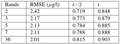
Bands RMSE (µg/l) r−2 r
Table 1. Statistics of the regression models: Root mean square error (RMSE), correlation coefficient r and coefficient of
determination r2.
the prototype 2012b was used to capture VIS/NIR spectral range images comprised from 36 wavelength bands from 500 nm to 875 nm. FPI images were captured from a manned single engine aircraft Cessna 172 Reims Rocket with an FPI camera using a flight height of about 2025 m above the mean sea level, provid-ing a GSD of 2 m. Block consisted of a total of 14 flight strips and 622 images. Forward overlaps were 75% and side overlaps were 53% in average. In situ reference variables of water quality were measured from a moving research vessel and seven water samples were taken for laboratory analysis for the calibration of the field data. The parameters measured were typical descriptors of eutrophication or otherwise important key elements of aquatic communities and health (Chl-a, BGA, NO23-N, Turbidity, TOC, NO23-N). Reference values of Chl-a consists of 650 measure-ments from different basins of Lohjanj¨arvi (A = 89 km2) with
sampling distance varying for 5 to 15 meter depending on vessel speed. Detailed description of measuring procedure is presented in (Erkkil¨a et al., 2017).
2.2 Data and algorithms
The range, mean and standard deviation of 650 measured Chl-a reference values are 1.93 - 26.06µg/l, 11.46µg/land 4.56µg/l, respectively. Multiple linear regression was used in deriving the model for predicting concentration of Chl-a by combination of DNs of different wavelengths measured by aerial hyperspectral imaging. The relation between measured Chl-a and regression estimated using all available 36 bands is presented in Figure 1. The combinations of 2, 3, 5 or 7 bands were selected using max-imum correlation with Chl-a concentration as an criterion; peak wavelengths for the best 2 bands combination are 693 and 850 nm, for 3 bands: 567, 682 and 850 nm, for 5 bands : 540, 567, 636, 682 and 850 nm and for 7 bands: 540, 567, 636, 662, 682, 733 and 850 nm. The basic statistics of the regression models applied to total 650 reference samples are presented in Table 1. Different numbers (8, 10, 12, 15, 20 and 30) of randomly selected Chl-a concentration samples were used as calibration subset in deriving the regression models and then models are applied to the rest of measurements used as validation subset. 50000 ran-domly selected combinations without duplicates were taken for each number of reference Chl-a samples. The standard deviation of Chl-a concentrations and average minimum distance of loca-tion of each selected combinaloca-tions were calculated. The average minimum distance is derived by determining minimum distance of each member of one selection from other members belonging to the same selection and then taking an average of these min-imum distances of members. Two dimensional probability and cumulative probability histograms were determined for present-ing and comparison of results.
Figure 1. Linear regression estimate of Chlorophyll a concentration when DNs of all bands are used as variables.
3. RESULTS
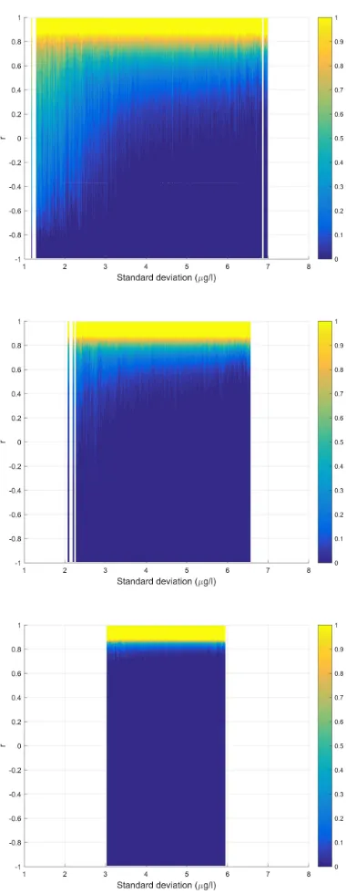
50000 numbers of 12 randomly selected reference Chl-a obser-vations have been used for deriving the regression model using the DN of 5 bands as an variables. The measured Chl-a concen-tration at all other of 650 reference location were considered as validation subset. The correlation coefficientr(Figures 2 and 4) is determined between the validation subset and Chl-a concentra-tion predicted by derived model at corresponding locaconcentra-tions. Four examples out of 50000 tests are illustrated in Figure 3. Therof all 50000 tests are presented as a function of standard deviation of Chl-a concentration of each 12 random samples by a scatter plot and two dimensional histogram in Figure 2. Probability his-togram and cumulative probability hishis-togram with respect torare presented in Figure 4. Only standard deviation bins, in which the sum of counts is over 30, are plotted. The cumulative histogram is presented for RMSE and correlation coefficient and RMSE are also presented as a function of average minimum distance param-eter describing the clustering of locations of 12 reference sam-ples. Correlation coefficients and errors at different cumulative probability levels, 0.01, 0.05, 0.1, 0.2 and 0.5, are presented in Figure 6. The higher standard deviation improves the correlation coefficient but does not ensure low RMSE; see an example pre-sented in Figure 3 (bottom left), where the correlation is fairly high (r = 0.77), but there is bias in the slope of predicted values, which explains the high error. Neither the high standard deviation nor large average minimum distance guarantee good predictabil-ity of the model with 99 % reliabilpredictabil-ity level (probabilpredictabil-ity = 0.01), when 12 reference samples are used in deriving the model with DN of 5 bands. However the situation improves and is stabilized significantly with reliability level 95 % if the standard deviation of reference values is adequately high.
The effect of number of independent variables on the r and RMSE is presented in Figures 9 and 10. With 30 reference locations, 2 and 3 band models approach their extreme values for r and RMSE presented in Table 1. They also require lower amount of refer-ence measurements to produce reliable model, but the result is more sensitive to standard deviation and clustering of reference samples than when DN of 5 or 7 bands are used. Probability to reach at least r = 0.7 is presented in Figure 11. For 5 bands model the r at least 0.7 is almost certain when 30 reference measures are used. If 12 reference samples are used, the probability is sig-nificantly dependent on standard deviation of reference values. With 2 and 3 band models the r at least 0.7 and RMSE lower than 4µg/l are achieved almost certainly if standard deviation of 12 reference measurements is roughly over 4.5µg/l (Figures 11 and 12).
Figure 2. Correlation coefficient between Chl-a estimates of linear regression model and in-situ Chl-a measurements. Model
is derived using 12 randomly selected reference Chl-a measurements (50000 random selections) and DN of five bands
as variables. Result is presented as a function of standard deviation of Chl-a concentration of 12 reference samples. Top:
scatter plot. Bottom: 2D histogram.
4. DISCUSSION AND CONCLUSION
In most studied cases the variation of correlations and errors de-pends only slightly on the clustering or variability of the reference measurements. The lower number of reference measurements or bands used in model increases this dependency. The effect is highest when correlation coefficient is studied as a function of standard deviation of reference measurements, while RMSE does not express equally notable trend. As can be expected, the higher number of observations (reference samples) improve the
Figure 3. Four examples of comparison of reference Chl-a concentrations and estimates derived by regression model based
on Chl-a measurements from 12 random locations (red circles and St.dev. values) are presented. The model is applied to the rest 638 Chl-a samples (black crosses, r and RMSE values).
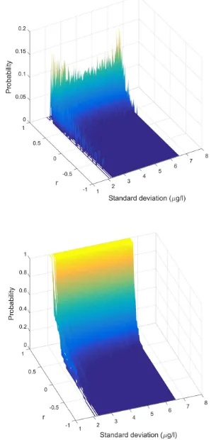
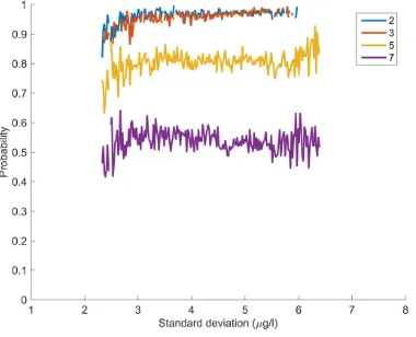
Figure 4. Probability histogram (top) and cumulative probability histogram (bottom) derived from data presented in Figure 1. The standard deviation bins for which the sum of counts is below 30
are rejected from probability histograms.
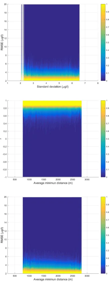
refer-Figure 5. Cumulative probability histograms derived using 5 bands and 12 randomly selected reference samples. The standard deviation bins (top) or average minimum distance bins (middle and bottom) for which the sum of counts is below 30 are
rejected from probability histograms.
ence samples to achieve same correlation coefficient with same confidence level as 2 or 3 band model reach with 12 reference measurements if their standard deviation of Chl-a concentrations is at least 4.5µg/l. The observations based on the empirical data of this study implies that better cost efficiency can be attained with 2 or 3 bands usage instead of 5 or 7 bands, when the amount of reference samples are wished to minimized. The more com-prehensive multi-criteria optimization could be used to estimate a more accurate cost minimum. It would also be interesting to test the same approach with other lake data (different lake or same lake at different seasons) to see if the trends and optima would
be the same; other optically active water quality parameters can be studied as well. The simple empirical approach combining re-mote sensing and traditional sampling methods may prove to be feasible when the goal is accurate long term monitoring of com-plex ecosystems.
5. ACKNOWLEDGEMENT
Study was partly funded by University of Jyvskyl and Tekes, the Finnish Funding Agency for Innovation (grants: 2208/31/2013 and 1711/31/2016).
REFERENCES
Bukata, R. P., 2013. Retrospection and introspection on remote sensing of inland water quality:like d´ej`a vu all over again. Jour-nal of Great Lakes Research39, pp. 2–5.
Erkkil¨a, A.-L., Lindfors, A., P¨ol¨onen, I., Honkavaara, E., Nurmi-nen, K., N¨asi, R. and OjaNurmi-nen, H., 2017. Water quality estimation in boreal lake by novel framing hyperspectral imaging.Submitted to Remote sensing of environment.
Honkavaara, E., Eskelinen, M. A., P¨ol¨onen, I., Saari, H., Ojanen, H., Mannila, R., Holmlund, C., Hakala, T., Litkey, P., Rosnell, T. et al., 2016. Remote sensing of 3-d geometry and surface mois-ture of a peat production area using hyperspectral frame cameras in visible to short-wave infrared spectral ranges onboard a small unmanned airborne vehicle (uav).
Honkavaara, E., Saari, H., Kaivosoja, J., P¨ol¨onen, I., Hakala, T., Litkey, P., M¨akynen, J. and Pesonen, L., 2013. Processing and assessment of spectrometric, stereoscopic imagery collected us-ing a lightweight uav spectral camera for precision agriculture. Remote Sensing5(10), pp. 5006–5039.
IOCCG, 2006. Remote Sensing of Inherent Optical Properties: Fundamentals, Tests of Algorithms, and Applications. Reports of the International Ocean Colour Coordinating Group, Vol. No. 5, IOCCG, Dartmouth, Canada.
Kutser, T., Herlevi, A., Kallio, K. and Arst, H., 2001. A hyper-spectral model for interpretation of passive optical remote sensing data from turbid lakes. Science of the Total Environment268(1), pp. 47–58.
M¨akynen, J., Saari, H., Holmlund, C., Mannila, R. and Antila, T., 2012. Multi-and hyperspectral uav imaging system for forest and agriculture applications. In: SPIE Defense, Security, and Sens-ing, International Society for Optics and Photonics, pp. 837409– 837409.
N¨asi, R., Honkavaara, E., Lyytik¨ainen-Saarenmaa, P., Blomqvist, M., Litkey, P., Hakala, T., Viljanen, N., Kantola, T., Tanhuanp¨a¨a, T. and Holopainen, M., 2015. Using uav-based photogrammetry and hyperspectral imaging for mapping bark beetle damage at tree-level.Remote Sensing7(11), pp. 15467–15493.
Palmer, S. C., Kutser, T. and Hunter, P. D., 2015. Remote sens-ing of inland waters: Challenges, progress and future directions. Remote Sensing of Environment157, pp. 1 – 8.
P¨ol¨onen, I., 2013. Discovering knowledge in various applications with a novel hyperspectral imager. Jyv¨askyl¨a studies in comput-ing; 1456-5390; 184.
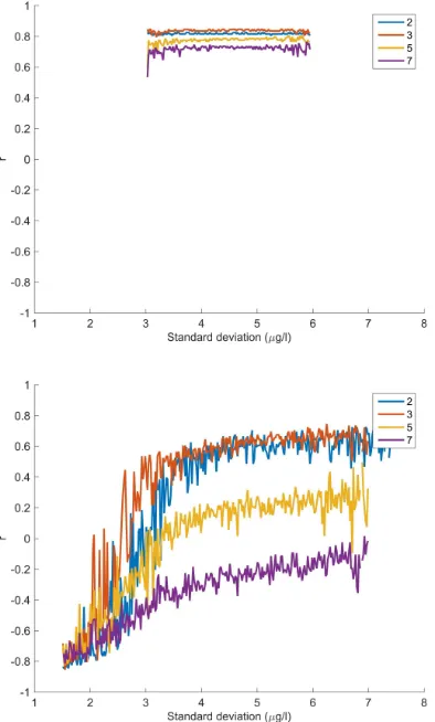
Figure6.Correlationcoefficientr(topandsecondfrombottom) androotmeansquareerror(RMSE)(secondfromtopand bottom)fordifferentprobabilitylevels.Allfigues:12randomly selectedreferencesamples,50000randomselectionand5bands.
Figure 7. Cumulative probability histograms derived using 5 bands and 8 (top), 12 (middle) and 30 (bottom) randomly selected reference samples. The standard deviation bins for
Figure8.Correlationcoefficientr(topandsecondfrombottom figures)andRMSE(secondfromtopandbottomfigures)for
differentnumberofrandomlyselectedmeasurements.All figures: 50000 random selection, probability level 0.05 and 5
bands.
Figure9.Correlationcoefficientr(topandsecondfrombottom figures)androotmeansquareerror(RMSE)(secondfromtop andbottomfigures)fordifferentnumberofwavelengthbandsas
Figure 10. Correlation coefficient r for different number of wavelength bands as variables. 30 (top) and 8 (bottom) randomly selected reference samples. Both figures: 50000
random selection and probability level 0.05.
Figure 11. Probability that the correlation coefficient r>0.7 for different number of randomly selected samples (top and middle
figures) and number of wavelength bands used as variables (bottom). 5 bands used for top and middle figures and 12 randomly selected reference measurements for bottom figure
Figure 12. The probability that the RMSE<4.0 is presented for different number of wavelength bands used as variables.12